SUSTAINABILITY - physical musings on the atmosphere #
v0.3 1.9.25 - THIS NOTEBOOK IS A WORK IN PROGRESS
Exercise structure#
A simple project usually goes along these lines:
Identify an area of interest (research question)
Find or collect materials (data acquisition)
Inquiry into the materials (analysis)
Assessment, critique (results and conclusions)
Further explanations as necessary (sources and discussion)
1. Research questions #
Observing and understanding climate change requires a global network. National weather stations, research institutes, universities and similar organisations all around the planet offer us a diverse selection of constantly updated observations.
First one should decide which variables they are looking at. Temperature, carbon dioxide and methane fractions in the air, ecosystem’s carbon fluxes, precipitation and winds et cetera.
How do the chosen variables evolve over time? What kinds of variation do they have? How does the observation site affect the results?
2. Data #
Let’s look at some materials on the carbon cycle from the ICOS-project. This multinational effort collects high-quality observations into their data portal in a collected and thus easily comparable format.
NOTE! The materials in the portal contain tens or hundreds of thousands of rows of data as well as dozens of cryptically named columns that contain the observations from various research stations. Each dataset includes a link to its source, where you can see the so-called metadata for what each column’s title means in more detail. In research, using various explanations and references like this is important to avoid confusion.
2.1 Tools#
# Let's import some important libraries.

import pandas as pd
import matplotlib.pyplot as plt
import numpy as np
2.2 Data - Hyytiälä, Middle-Finland#
# Methane concentration
# Hyytiälä 67.2 m CH4 2016-12-13–2023-03-31
# https://meta.icos-cp.eu/objects/XRJWd0QZw0wKGjXZnspH20t5

HyyCH4 = pd.read_csv("https://raw.githubusercontent.com/opendata-education/Tyopajat/main/materiaali/data/HyyCH4.csv",
                     parse_dates = ["TIMESTAMP"])

# Carbon dioxide concentration
# Hyytiälä 67.2 m CO2 2016-12-13–2023-03-31
# https://meta.icos-cp.eu/objects/9Y6WV_HjpEVbbc-lq_FE9qV8

HyyCO2 = pd.read_csv("https://raw.githubusercontent.com/opendata-education/Tyopajat/main/materiaali/data/HyyCO2.csv",
                     parse_dates = ["TIMESTAMP"])

# Meteorological observations
# Hyytiälä 67.2 m ICOS ATC Meteo 2017-12-31–2022-12-31
# https://meta.icos-cp.eu/objects/zdx_A4ariX25X6Pu8DUG_vE1

HyyMeteo = pd.read_csv("https://raw.githubusercontent.com/opendata-education/Tyopajat/main/materiaali/data/HyyMeteo.csv",
                       parse_dates = ["TIMESTAMP"])

# Fluxes
# Hyytiälä FLUXNET-archive 1996-2020
# https://meta.icos-cp.eu/objects/4F2-9d7QV9A0SlL2pIaRxsJP

HyyGPP = pd.read_csv("https://raw.githubusercontent.com/opendata-education/Tyopajat/main/materiaali/data/HyyFluxGPP.csv",
                     parse_dates = ["TIMESTAMP"])
HyyNEE = pd.read_csv("https://raw.githubusercontent.com/opendata-education/Tyopajat/main/materiaali/data/HyyFluxNEE.csv",
                     parse_dates = ["TIMESTAMP"]) # this one also includes temperature
2.3 Data - Utö, Baltic Sea, Finnish archipelago#
# Methane concentration
# Atmospheric CH4 product, Utö - Baltic sea (57.0 m) 2012-03-23–2023-03-31
# https://meta.icos-cp.eu/objects/0QpkTakURubEz9vnSxkAIL3j

UtCH4 = pd.read_csv("https://raw.githubusercontent.com/opendata-education/Tyopajat/main/materiaali/data/UtCH4.csv",
                    parse_dates = ["TIMESTAMP"])

# Carbon dioxide concentration
# Atmospheric CO2 product, Utö - Baltic sea (57.0 m) 2012-03-23–2023-03-31
# https://meta.icos-cp.eu/objects/Gfcb8rZBPxZQNJgm7qiwAcYz

UtCO2 = pd.read_csv("https://raw.githubusercontent.com/opendata-education/Tyopajat/main/materiaali/data/UtCO2.csv",
                    parse_dates = ["TIMESTAMP"])

# Meteorological observations
# Utö 58 m ICOS ATC Meteo 2018-12-12–2023-03-31
# https://meta.icos-cp.eu/objects/Q9In1Q-KI-HrxDHlrHytOCOd

UtMeteo = pd.read_csv("https://raw.githubusercontent.com/opendata-education/Tyopajat/main/materiaali/data/UtMeteo.csv",
                      parse_dates = ["TIMESTAMP"])
2.4 Data - Pallas and Kenttärova, Northern Finland#
# Atmospheric CH4 product, Pallas (12.0 m)
# 2004-02-11–2023-03-31
# https://meta.icos-cp.eu/objects/ATqgqugIHsWAIXKZgEq2QkKz

PalCH4 = pd.read_csv("https://raw.githubusercontent.com/opendata-education/Tyopajat/main/materiaali/data/PalCH4.csv",
                     parse_dates = ["TIMESTAMP"])

# Atmospheric CO2 product, Pallas (12.0 m)
# 1998-07-01–2023-03-31
# https://meta.icos-cp.eu/objects/sp32Z270ruWRU847KagynNOK

PalCO2 = pd.read_csv("https://raw.githubusercontent.com/opendata-education/Tyopajat/main/materiaali/data/PalCO2.csv",
                     parse_dates = ["TIMESTAMP"])

# Fluxnet Product, Kenttarova
# 2017-12-31–2020-12-31
# https://meta.icos-cp.eu/objects/vXcr9a7FPpBA3_Tg5X2gT1xo

KenFlux1 = pd.read_csv("https://raw.githubusercontent.com/opendata-education/Tyopajat/main/materiaali/data/KenFlux1.csv",
                       parse_dates = ["TIMESTAMP"])

# ETC L2 Fluxnet (half-hourly), Kenttarova
# 2019-12-31–2022-12-31
# https://meta.icos-cp.eu/objects/aqULa_iF0GDVTc4_AUb7h-nN

KenFlux2 = pd.read_csv("https://raw.githubusercontent.com/opendata-education/Tyopajat/main/materiaali/data/KenFlux2.csv",
                       parse_dates = ["TIMESTAMP"])
/tmp/ipykernel_2467/2414738136.py:19: DtypeWarning: Columns (7,11,13,25) have mixed types. Specify dtype option on import or set low_memory=False.
  KenFlux1 = pd.read_csv("https://raw.githubusercontent.com/opendata-education/Tyopajat/main/materiaali/data/KenFlux1.csv",
2.5 Data - Karlsruhe, Germany#
# Methane concentration
# Karlsruhe 60 m CH4 2016-12-16–2023-03-31
# https://meta.icos-cp.eu/objects/lO1I16P7gM7zloZbzWLSur02

KarlCH4 = pd.read_csv("https://raw.githubusercontent.com/opendata-education/Tyopajat/main/materiaali/data/KarlCH4.csv",
                      parse_dates = ["TIMESTAMP"])

# Carbon dioxide concentration
# Karlsruhe 60 m CO2 2016-12-16–2023-03-31
# https://meta.icos-cp.eu/objects/vXTxJscV4CHFfaljH9KQ5pty

KarlCO2 = pd.read_csv("https://raw.githubusercontent.com/opendata-education/Tyopajat/main/materiaali/data/KarlCO2.csv",
                      parse_dates = ["TIMESTAMP"])

# Meteorological observations
# Karlsruhe 60 m ICOS ATC Meteo 2019-08-01–2023-03-31
# https://meta.icos-cp.eu/objects/rJGDmG0anqNeRrPyLBuog258

KarlMeteo = pd.read_csv("https://raw.githubusercontent.com/opendata-education/Tyopajat/main/materiaali/data/KarlMeteo.csv",
                        parse_dates = ["TIMESTAMP"])
2.6 Data - Castelporziano 2, Italy#
# Fluxes
# Castelporziano ETC L2 Fluxnet 2020-12-31–2023-10-31
# https://meta.icos-cp.eu/objects/DZcO_1NvbH4wRqTcxnNVKd47

CasFlux = pd.read_csv("https://raw.githubusercontent.com/opendata-education/Tyopajat/main/materiaali/data/CasFlux.csv",
                      parse_dates = ["TIMESTAMP"])

# Meteorological observations
# Castelporziano ETC L2 Meteo 2020-12-31–2023-10-31
# https://meta.icos-cp.eu/objects/b9jFmI9WtonRGMRRsWOeBQK9

CasMeteo = pd.read_csv("https://raw.githubusercontent.com/opendata-education/Tyopajat/main/materiaali/data/CasMeteo.csv",
                       parse_dates = ["TIMESTAMP"])
/tmp/ipykernel_2467/2867836255.py:5: DtypeWarning: Columns (11,13,25) have mixed types. Specify dtype option on import or set low_memory=False.
  CasFlux = pd.read_csv("https://raw.githubusercontent.com/opendata-education/Tyopajat/main/materiaali/data/CasFlux.csv",
2.7 Data - Izaña, Spain (Tenerife)#
# Methane concentration
# Atmospheric CH4 product, Izaña (29.0 m) 1984-01-01–2023-03-31
# https://meta.icos-cp.eu/objects/j_qLA35m18_V9HXmKXNTtV1d

IzaCH4 = pd.read_csv("https://raw.githubusercontent.com/opendata-education/Tyopajat/main/materiaali/data/IzaCH4.csv",
                     parse_dates = ["TIMESTAMP"])

# Carbon dioxide concentration
# Atmospheric CO2 product, Izaña (29.0 m) 2007-01-19–2023-03-31
# https://meta.icos-cp.eu/objects/pinswiNsT4yB9YSX5O-TlAYD

IzaCO2 = pd.read_csv("https://raw.githubusercontent.com/opendata-education/Tyopajat/main/materiaali/data/IzaCO2.csv",
                     parse_dates = ["TIMESTAMP"])

# Meteorological observations
# 1996-01-01-2023-12-21
# https://meteostat.net/en/station/60010
# (retrieved from another source, as the station is relatively new to the ICOS network
# despite being well established on its own)

IzaMet = pd.read_csv("https://raw.githubusercontent.com/opendata-education/Tyopajat/main/materiaali/data/IzaMet.csv",
                     parse_dates = ["date"])
3. Analysis #
Let’s take a look at the data contained in the materials defined above. The following example uses observations from Hyytiälä, but you can analyse the other stations just as well by changing the names of the variables (by opening, say, ‘CasFlux’ instead).
3.1 A peek into the materials#
# Let's see what the information stored into the variables looks like.

HyyCO2
| Stdev | TIMESTAMP | co2 | |
|---|---|---|---|
| 0 | -9.990 | 2016-12-13 00:00:00 | NaN |
| 1 | -9.990 | 2016-12-13 01:00:00 | NaN |
| 2 | -9.990 | 2016-12-13 02:00:00 | NaN |
| 3 | -9.990 | 2016-12-13 03:00:00 | NaN |
| 4 | 0.011 | 2016-12-13 04:00:00 | 411.702 |
| ... | ... | ... | ... |
| 63966 | 0.238 | 2024-03-31 19:00:00 | 425.800 |
| 63967 | 0.101 | 2024-03-31 20:00:00 | 426.426 |
| 63968 | 0.264 | 2024-03-31 21:00:00 | 426.438 |
| 63969 | 0.614 | 2024-03-31 22:00:00 | 427.758 |
| 63970 | 0.375 | 2024-03-31 23:00:00 | 428.537 |
63971 rows × 3 columns
# Let's make the simplest graph we can from the data in one column.

plt.plot(HyyCO2["TIMESTAMP"], HyyCO2["co2"])
plt.show()
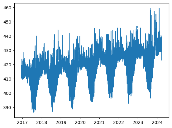
Are there any repeating patterns you can discern in the graph? What is happening?
3.2 A more detailed look#
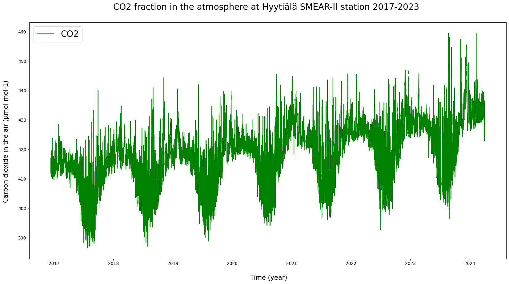
# Let's add some formatting into the graph.

plt.figure(figsize = (20, 10))

plt.plot(HyyCO2["TIMESTAMP"], HyyCO2["co2"], label = "CO2", color = "green")

plt.ylabel("Carbon dioxide in the air (µmol mol-1) \n", fontsize = 15)
plt.xlabel("\n Time (year)", fontsize = 15)
plt.title("CO2 fraction in the atmosphere at Hyytiälä SMEAR-II station 2017-2023 \n", fontsize = 20)
plt.legend(loc = "upper left", fontsize = 20)

plt.show()
# Showing multiple quantities at the same time.

plt.figure(figsize = (20, 10))

plt.subplot(311)
plt.plot(HyyCO2["TIMESTAMP"], HyyCO2["co2"], label = "CO2", c = "g")
plt.ylabel("Concentration in the air \n (µmol mol-1) \n", fontsize = 10)
plt.legend(loc = "upper left", fontsize = 20)

plt.title("Molecular fractions in the atmosphere at Hyytiälä SMEAR-II station 2017-2023 \n", fontsize = 20)

plt.subplot(312)
plt.plot(HyyCH4["TIMESTAMP"], HyyCH4["ch4"], label = "CH4", c = "b")
plt.ylabel("Concentration in the air \n (nmol mol-1) \n", fontsize = 10)
plt.legend(loc = "upper left", fontsize = 20)

plt.subplot(313)
plt.plot(HyyMeteo["TIMESTAMP"], HyyMeteo["AT"], label = "Temperature", c = "cyan")
plt.ylabel("Air temperature(°C) \n", fontsize = 10)
plt.legend(loc = "upper left", fontsize = 20)

plt.xlabel("\n Time (year)", fontsize = 15)
plt.show()
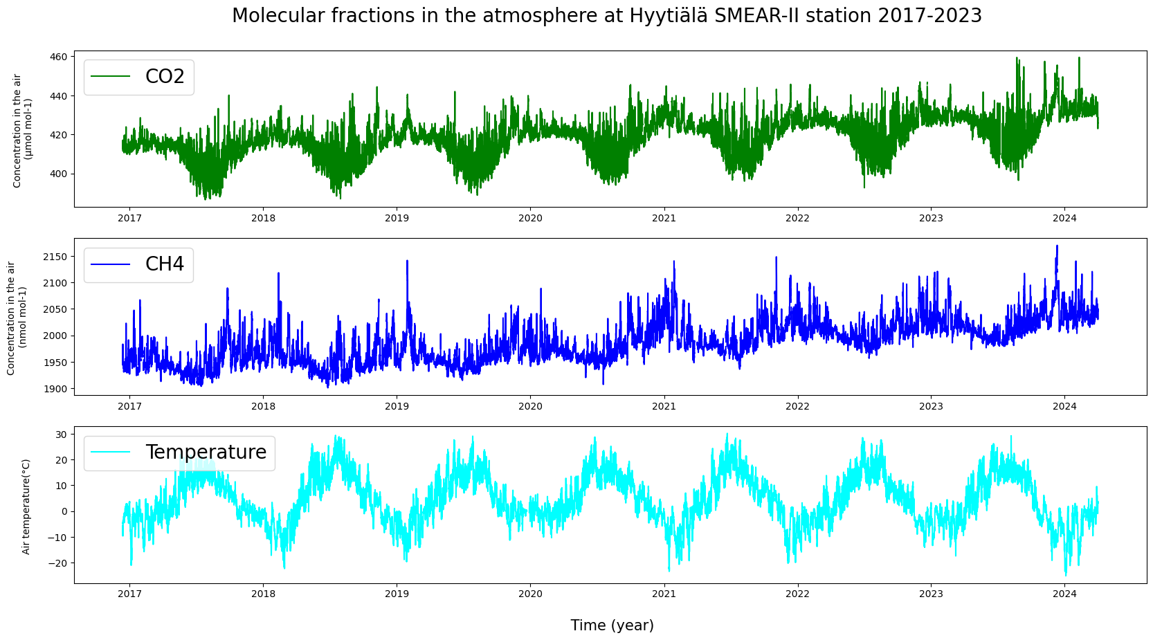
Are the quantities in the graphs dependent on each other? Do they exhibit any similarities or deviations from each other?
# Let's repeat the above for ecosystemic action over a bit longer period as well. Let's add a zero line for clarity.

plt.figure(figsize = (20, 10))

plt.subplot(311)
plt.plot(HyyNEE["TIMESTAMP"], HyyNEE["NEE_VUT_REF"], label = "NEE", c = "g")
plt.axhline(y = 0, color = 'y', linestyle = 'dashed')
plt.ylabel("Net Ecosystem Exchange \n (µmol m-2 s-1) \n", fontsize = 10)
plt.legend(loc = "upper left", fontsize = 20)

plt.title("Carbon fluxes in the forest at Hyytiälä SMEAR-II station 1996-2020 \n", fontsize = 20)

plt.subplot(312)
plt.plot(HyyGPP["TIMESTAMP"], HyyGPP["GPP_DT_VUT_REF"], label = "GPP DT", c = "b", alpha = 0.5)
plt.plot(HyyGPP["TIMESTAMP"], HyyGPP["GPP_NT_VUT_REF"], label = "GPP NT", c = "orange", alpha = 0.5)
plt.axhline(y = 0, color = 'y', linestyle = 'dashed')
plt.ylabel("CO2 Gross Primary Production \n (µmol m-2 s-1) \n", fontsize = 10)
plt.legend(loc = "upper left", fontsize = 20)

plt.subplot(313)
plt.plot(HyyNEE["TIMESTAMP"], HyyNEE["TA_F"], label = "Temperature", c = "cyan")
plt.axhline(y = 0, color = 'y', linestyle = 'dashed')
plt.ylabel("Air temperature (°C) \n", fontsize = 10)
plt.legend(loc = "upper left", fontsize = 20)

plt.xlabel("\n Time (year)", fontsize = 15)
plt.show()
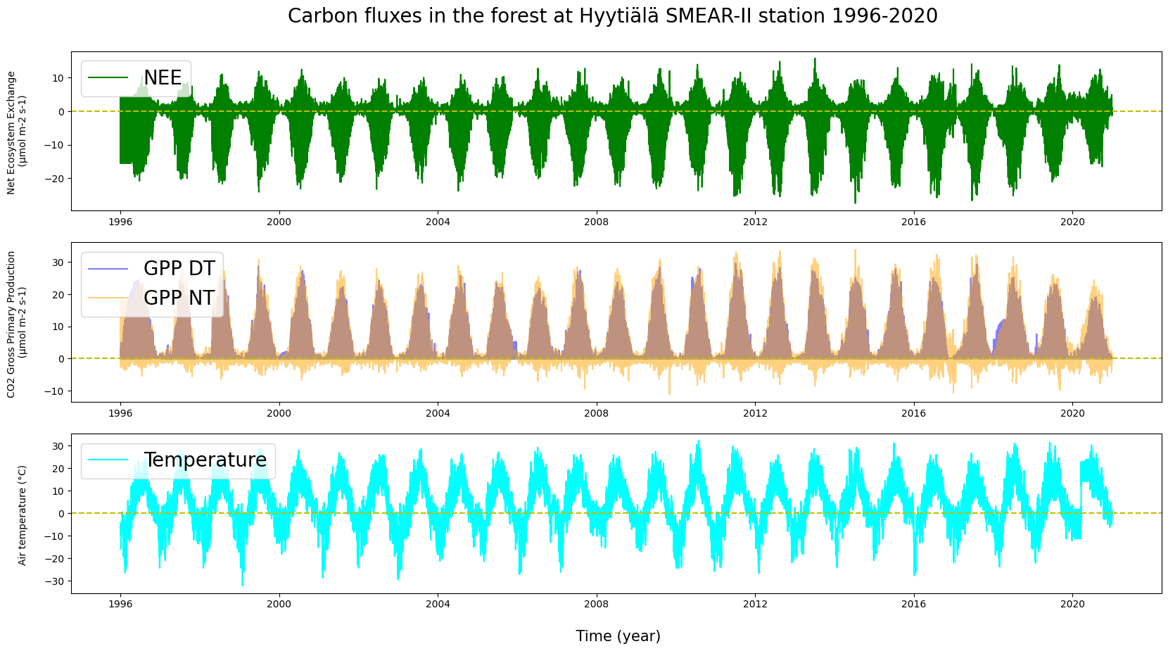
Can you see any variation between the years or the seasons?
3.3. Understanding data requires working with it#
When we’re looking at graphs, it’s worth bearing in mind how frequently observations have been taken and how many of them there are. The data you’ve seen above has been collected hourly or more frequently, which might lead to some needless detail in your graphs. For the sake of clarity, it is often necessary to split, categorise, average or otherwise edit the original data and try to pry out certain statistical variables that emerge from the raw numbers in order to move from pure data to meaningful information.
# Let's edit an existing variable. We'll take the collated timestamps in the data, split them into their constituents and save
# them in new columns inside the same variable. This will make it easier to select certain parts of the data, such as "all
# summer months only".

# For example, the first ten rows in our CO2 table were:
print("HyyCO2 in the beginning: ")
print(HyyCO2.head(10))

# Adding columns by digging the information out of the timestamp in their own columns:

HyyCO2['DATE'] = pd.to_datetime(HyyCO2['TIMESTAMP']).dt.date
HyyCO2['DATE'] = pd.to_datetime(HyyCO2['DATE'])                # Correcting the date-format into a datetime-format.
HyyCO2['YY'] = pd.to_datetime(HyyCO2['TIMESTAMP']).dt.year
HyyCO2['MM'] = pd.to_datetime(HyyCO2['TIMESTAMP']).dt.month
HyyCO2['DD'] = pd.to_datetime(HyyCO2['TIMESTAMP']).dt.day
HyyCO2['HH'] = pd.to_datetime(HyyCO2['TIMESTAMP']).dt.hour

print("HyyCO2 after a small edit: ")
print(HyyCO2.head(10))
HyyCO2 in the beginning:
   Stdev           TIMESTAMP      co2
0 -9.990 2016-12-13 00:00:00      NaN
1 -9.990 2016-12-13 01:00:00      NaN
2 -9.990 2016-12-13 02:00:00      NaN
3 -9.990 2016-12-13 03:00:00      NaN
4  0.011 2016-12-13 04:00:00  411.702
5  0.185 2016-12-13 05:00:00  411.800
6  2.023 2016-12-13 06:00:00  414.534
7  0.222 2016-12-13 07:00:00  416.558
8  0.338 2016-12-13 08:00:00  416.367
9  0.401 2016-12-13 09:00:00  417.059
HyyCO2 after a small edit:
   Stdev           TIMESTAMP      co2       DATE    YY  MM  DD  HH
0 -9.990 2016-12-13 00:00:00      NaN 2016-12-13  2016  12  13   0
1 -9.990 2016-12-13 01:00:00      NaN 2016-12-13  2016  12  13   1
2 -9.990 2016-12-13 02:00:00      NaN 2016-12-13  2016  12  13   2
3 -9.990 2016-12-13 03:00:00      NaN 2016-12-13  2016  12  13   3
4  0.011 2016-12-13 04:00:00  411.702 2016-12-13  2016  12  13   4
5  0.185 2016-12-13 05:00:00  411.800 2016-12-13  2016  12  13   5
6  2.023 2016-12-13 06:00:00  414.534 2016-12-13  2016  12  13   6
7  0.222 2016-12-13 07:00:00  416.558 2016-12-13  2016  12  13   7
8  0.338 2016-12-13 08:00:00  416.367 2016-12-13  2016  12  13   8
9  0.401 2016-12-13 09:00:00  417.059 2016-12-13  2016  12  13   9
# Calculating monthly averages.

AVG = HyyCO2.groupby(["MM"]).mean(numeric_only = True)

print(AVG["co2"])

k = ["Jan", "Feb", "Mar", "Apr", "May", "Jun", "Jul", "Aug", "Sep", "Oct", "Nov", "Dec"]

plt.figure(figsize = (20, 10))
plt.plot(k, AVG["co2"], c = "y")
plt.scatter(k, AVG["co2"], c = "red", label = "CO2")

plt.ylabel("Concentration in the air (µmol mol-1) \n", fontsize = 15)
plt.xlabel("\n Time (month)", fontsize = 15)
plt.title("Carbon dioxide fraction in the atmosphere at Hyytiälä SMEAR-II station, monthly average 2017-2023 \n", fontsize = 20)
plt.legend(loc = "center right", fontsize = 15)

plt.show()
MM
1     424.377297
2     424.810247
3     423.362963
4     420.545571
5     417.881080
6     411.357302
7     406.461138
8     407.401265
9     412.127879
10    417.971593
11    424.054693
12    425.309426
Name: co2, dtype: float64
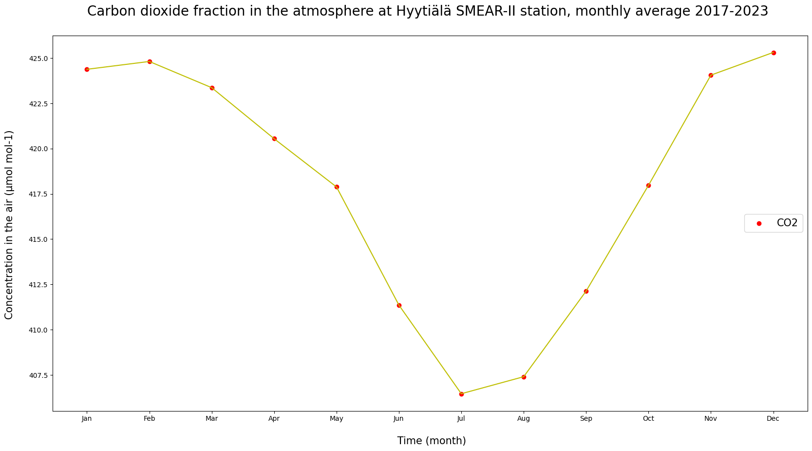
How does the averaged graph look compared to the original observations?
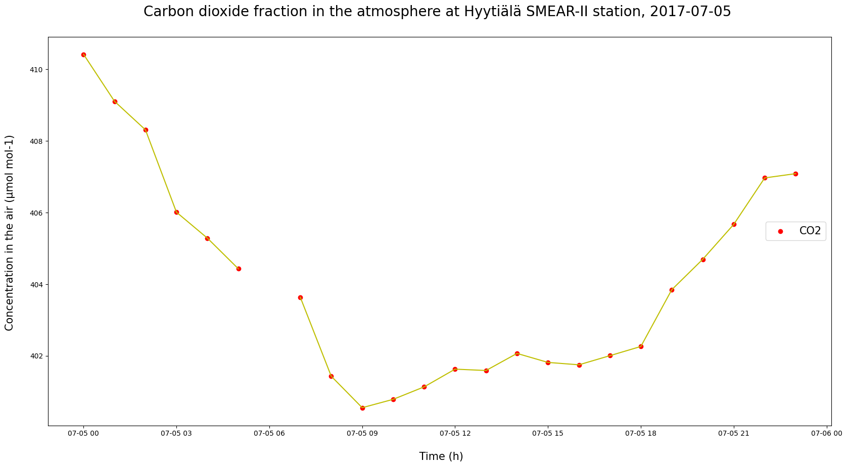
# Longer datasets can give us a better picture of seasonal variations.
# What about shorter periods, like within a day?

d = '2017-07-05'
dat = HyyCO2.query("DATE == @d")

plt.figure(figsize = (20, 10))
plt.plot(dat["TIMESTAMP"], dat["co2"], c = "y")
plt.scatter(dat["TIMESTAMP"], dat["co2"], c = "red", label = "CO2")

plt.ylabel("Concentration in the air (µmol mol-1) \n", fontsize = 15)
plt.xlabel("\n Time (h)", fontsize = 15)
plt.title(f"Carbon dioxide fraction in the atmosphere at Hyytiälä SMEAR-II station, {d} \n", fontsize = 20)
plt.legend(loc = "center right", fontsize = 15)

plt.show()
/tmp/ipykernel_2467/4083719619.py:5: FutureWarning: The behavior of 'isin' with dtype=datetime64[ns] and castable values (e.g. strings) is deprecated. In a future version, these will not be considered matching by isin. Explicitly cast to the appropriate dtype before calling isin instead.
  dat = HyyCO2.query("DATE == @d")
# Or between given dates?
# Try to switch the graphed period over two days, a week or a month.

a = '2017-07-05'
b = '2017-07-09'
cut = HyyCO2.query("DATE >= @a & DATE < @b")

plt.figure(figsize = (20, 10))
plt.plot(cut["TIMESTAMP"], cut["co2"], c = "y")
plt.scatter(cut["TIMESTAMP"], cut["co2"], c = "red", label = "CO2")

plt.ylabel("Concentration in the air (µmol mol-1) \n", fontsize = 15)
plt.xlabel("\n Time (h)", fontsize = 15)
plt.title(f"Carbon dioxide fraction at Hyytiälä SMEAR-II station, between {a} and {b} \n", fontsize = 20)
plt.legend(loc = "center right", fontsize = 15)

plt.show()
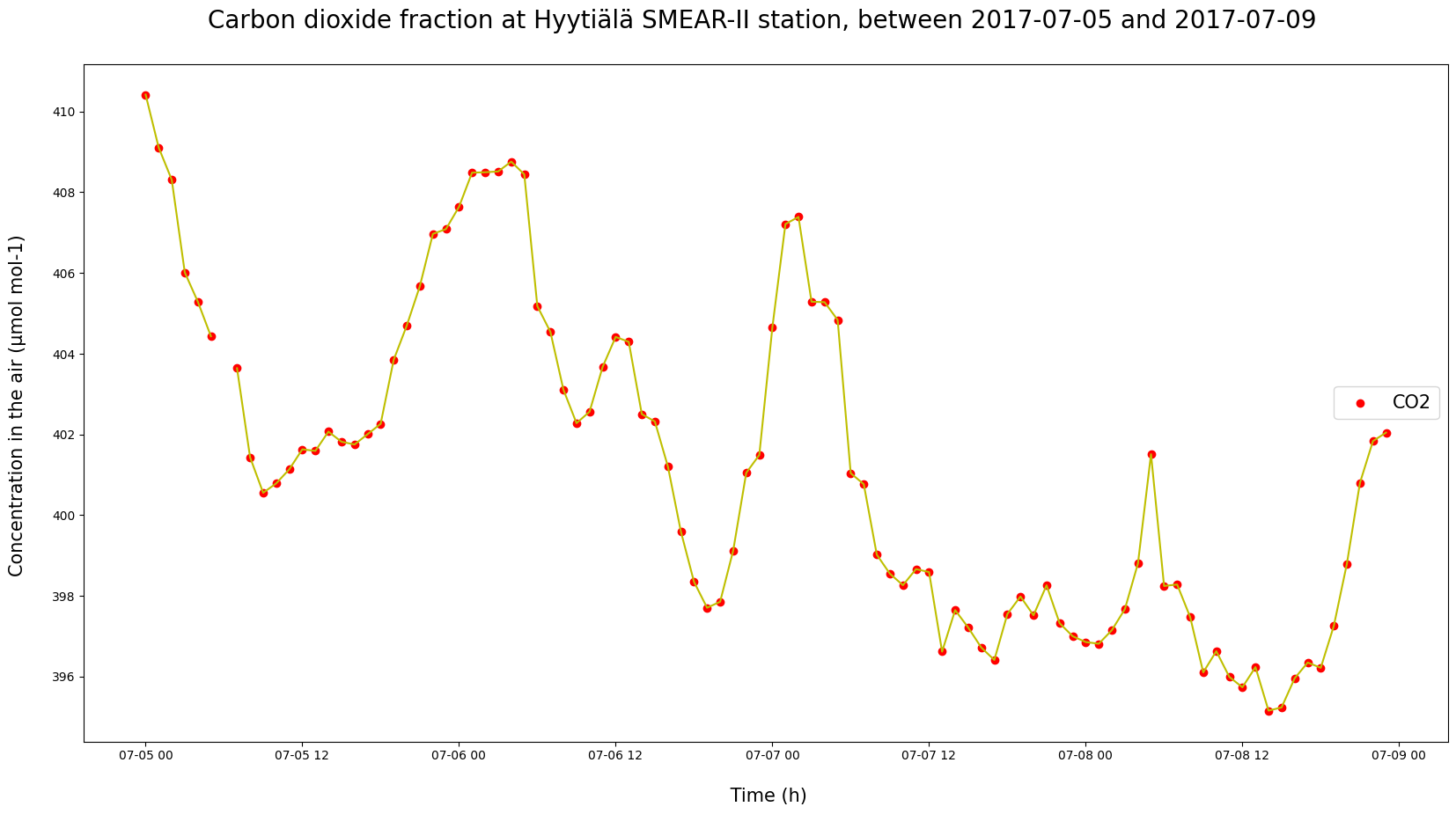
What kind of differences can you find between days within the same season? Do the shapes or sizes of daily variation change between seasons?
3.4 Finding connections requires using multiple sources and observed quantities#
# Daily CO2-levels, temperatures, rainfall, short-wave radiation, GPP?
# Try here.
3.5 Comparisons between various stations to find out regional differences#
# For example, Hyytiälä v. Izana

bott = "2016-01-01"
top = "2024-01-01"

bott = pd.to_datetime(bott)
top = pd.to_datetime(top)

plt.figure(figsize = (20, 10))

ax1 = plt.subplot(211)
plt.plot(HyyCO2["TIMESTAMP"], HyyCO2["co2"], label = "Hyytiälä", c = "g", alpha = 0.5)
plt.plot(IzaCO2["TIMESTAMP"], IzaCO2["co2"], label = "Izana", c = "b", alpha = 0.5)
plt.ylabel("Concentration in the air \n (µmol mol-1) \n", fontsize = 10)
plt.legend(loc = "upper left", fontsize = 20)
plt.xlim(bott, top)

plt.title(f"CO2 fractions and temperatures in the atmosphere between {bott} - {top} \n", fontsize = 20)

plt.subplot(212, sharex = ax1)
plt.plot(HyyMeteo["TIMESTAMP"], HyyMeteo["AT"], label = "Hyytiälä", c = "cyan", alpha = 0.7)
plt.plot(IzaMet["date"], IzaMet["tavg"], label = "Izana", c = "red", alpha = 0.5)
plt.axhline(y = 0, color = 'y', linestyle = 'dashed')
plt.ylabel("Air temperature (°C) \n", fontsize = 10)
plt.legend(loc = "upper left", fontsize = 20)

plt.xlabel("\n Time (year)", fontsize = 15)
plt.show()
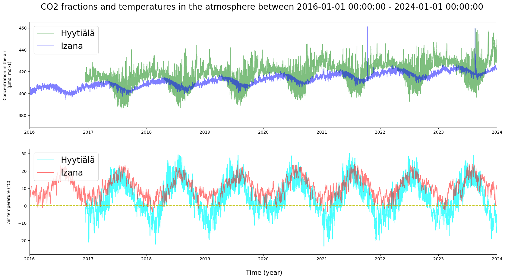
How do the observations in Finland and at the Canary Islands differ? Do they contain momentary deviations? Does it make a difference, that the temperature values in the Izaña data are daily averages?
# The individual observations seem to see-saw up and down. Let's fit a trend line in there to get a general idea of them.

plt.figure(figsize = (20, 10))

# Observation data

plt.plot(HyyCO2["TIMESTAMP"], HyyCO2["co2"], label = "Hyytiälä", c = "g", alpha = 0.5)
plt.plot(IzaCO2["TIMESTAMP"], IzaCO2["co2"], label = "Izana", c = "b", alpha = 0.5)

# Hyytiälä trend

x = np.arange(HyyCO2['TIMESTAMP'].size)
y = HyyCO2["co2"].copy()
y[np.isnan(y)] = y[~np.isnan(y)].mean()

z = np.polyfit(x, y, 1)
p = np.poly1d(z)
plt.plot(HyyCO2['TIMESTAMP'], p(x), c = "black", linestyle = "dashed", label = "Hyytiälä", alpha = 0.7)

# Izaña trend

q = np.arange(IzaCO2['TIMESTAMP'].size)
w = IzaCO2["co2"].copy()
w[np.isnan(w)] = w[~np.isnan(w)].mean()

v = np.polyfit(q, w, 1)
pf = np.poly1d(v)
plt.plot(IzaCO2['TIMESTAMP'], pf(q), "r--", label = "Izana", alpha = 0.7)

# Labels

plt.xlabel("\n Time (year)", fontsize = 20)
plt.ylabel("Concentration in the air (µmol mol-1) \n", fontsize = 20)
plt.legend(loc = "upper left", fontsize = 20)

plt.title("CO2 fraction trend at the measuring stations between 2008-2023 \n", fontsize = 20)
plt.show()

print(f"Hyytiälä's trendline equation: y = {z[0]}*x + {z[1]}")
print(f"Izaña's trendline equation: y = {v[0]}*x + {v[1]}")
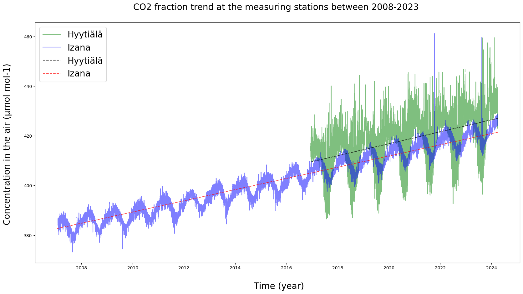
Hyytiälä's trendline equation: y = 0.0002745232373427903*x + 409.4827833577826
Izaña's trendline equation: y = 0.000257227561759758*x + 382.68451850415585
Are there observable trends in the data? Do the trends differ based on location or other factors between the stations? What needs to be accounted for in reading the equations?
4. Results and conclusions #
- discussion on the implications -
5. Sources #
- discussion on the stations or any further inquiries performed -