Statistics with the CMS Open Data
Contents
Statistics with the CMS Open Data#
With Python it is easy to calculate statistical values for the CMS Open Data. In this notebook we will learn how to calculate the mean, the variance, and the standard deviation.
We will use the particle physics data collected by the CMS detector. In the file Jpsimumu_Run2011A.csv there are selected events from the CMS primary dataset [1] with the specific criteria [2].
We will start the calculation by importing the necessary Python modules and getting the data from the file.
[1] CMS collaboration (2016). DoubleMu primary dataset in AOD format from RunA of 2011 (/DoubleMu/Run2011A-12Oct2013-v1/AOD). CERN Open Data Portal. DOI: 10.7483/OPENDATA.CMS.RZ34.QR6N.
[2] Thomas McCauley (2016). Jpsimumu. Jupyter Notebook file. https://github.com/tpmccauley/cmsopendata-jupyter/blob/hst-0.1/Jpsimumu.ipynb.
Settings and plotting the histogram#
# Import the needed modules. Pandas is for the data-analysis, numpy for scientific calculation,
# and matplotlib.pyplot for making plots. Modules are named as pd, np, and plt, respectively.
import pandas as pd
import numpy as np
import matplotlib.pyplot as plt

# Jupyter Notebook uses "magic functions". With this function it is possible to plot
# the histogram straight to notebook.
%matplotlib inline

# Create a new DataFrame structure from the file "Jpsimumu_Run2011A.csv"
dataset = pd.read_csv('../../Data/Jpsimumu_Run2011A.csv')

# Create a Series structure (basically a list) and name it "inv_mass".
# Save the column "M" from "dataset" to the variable "inv_mass".
inv_mass = dataset['M']
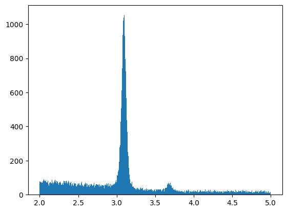
We will plot the histogram of the invariant masses of our data:
plt.hist(inv_mass, bins=500)
plt.show()
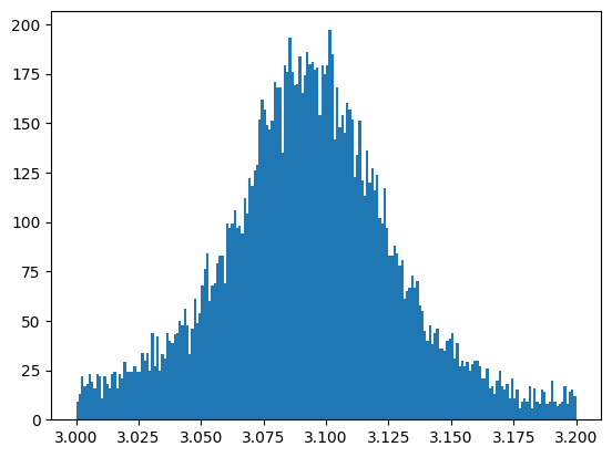
We will focus on the data around the first peak and save the values in the variable “peakdata”. Place the invariant masses in our range into the variable “peak_invmass”.
peakdata = dataset[(inv_mass>3.0) & (inv_mass<3.2)]
peak_invmass = peakdata['M']
plt.hist(peak_invmass, bins=200)
plt.show()
Mean \(\bar x\)#
The mean can be easily calculated with the function mean( ) of the numpy module. Let us calculate the mean of the invariant masses of the whole dataset:
mean_masses = np.mean(inv_mass)
print(mean_masses)
3.084373634453781
Let us compare it to the mean of the invariant masses near the peak:
mean_peakmasses = np.mean(peak_invmass)
print(mean_peakmasses)
3.0934255293362805
Variance \(\sigma^2\)#
The variance is determined by the equation
With Python the variance can be calculated with the function var( ) of the numpy module. Let us do that for the whole dataset.
variance = np.var(inv_mass)
print(variance)
0.3921691908895594
and for the peak
peak_variance = np.var(peak_invmass)
print(peak_variance)
0.001290814368485398
Standard deviation \(\sigma\)#
Because the standard deviation is the square root of the variance, we can calculate the standard deviation with the function sqrt( ) of the numpy module. The function sqrt( ) calculates the square root for the given value. Once again, for the whole dataset we get:
sd = np.sqrt(variance)
print(sd)
0.6262341342417861
and for the peak
sd_peak = np.sqrt(peak_variance)
print(sd_peak)
0.03592790515025052
Why are there differences in the statistical values? How do you know which way is the right one for each occasion?