Creating a normal distribution fit of transverse momentum and pseudorapidity

The point of this exercise is to learn to create a normal distribution fit for the data, and to learn about transverse momentum and pseudorapidity (and how they are linked together). The data used is open data released by the CMS experiment.

The fit

Let us begin by loading the needed modules, data, and creating a histogram of the data to see the more interesting points (the area for which we want to create the fit).

# This is needed to create the fit
from scipy.stats import norm

import pandas as pd
import numpy as np
import matplotlib.mlab as mlab
import matplotlib.pyplot as plt

# Let us use Dimuon_DoubleMu.csv 
data = pd.read_csv('http://opendata.cern.ch/record/545/files/Dimuon_DoubleMu.csv')

# And save the invariant masses to iMass
iMass = data['M']

# Plus draw the histogram
n, bins, patches = plt.hist(iMass, 300, facecolor='g')
plt.xlabel('Invariant Mass (GeV)')
plt.ylabel('Amount')
plt.title('Histogram of the invariant masses')

plt.show()

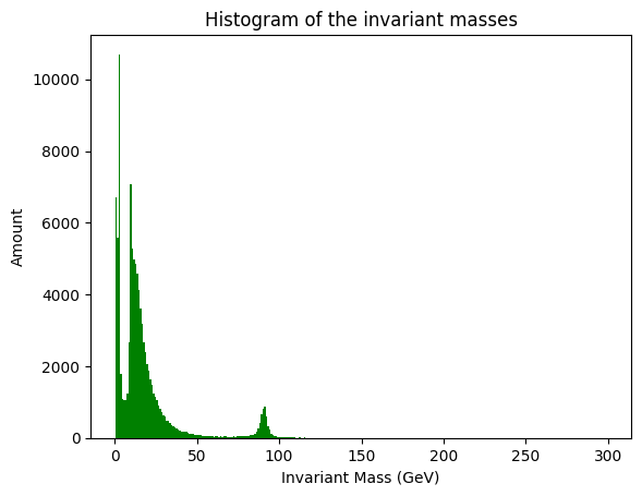
Let us take a closer look of the bump around 90GeVs.

min = 85
max = 97

# Let us crop the area. croMass now includes all the masses between the values of min and max
croMass = iMass[(min < iMass) & (iMass < max)]

# Calculate the mean (µ) and standard deviation (sigma) of normal distribution using the norm.fit function from scipy
(mu, sigma) = norm.fit(croMass)

# Histogram of the cropped data. Note that the data is normalized (density = 1)
n, bins, patches = plt.hist(croMass, 300, density = 1, facecolor='g')

#mlab.normpdf calculates the normal distribution's y-value with given µ and sigma
# let us also draw the distribution to the same image with histogram
y = norm.pdf(bins, mu, sigma)
l = plt.plot(bins, y, 'r-.', linewidth=3)


plt.xlabel('Invarian Mass(GeV)')
plt.ylabel('Probability')
plt.title(r'$\mathrm{Histogram \ and\ fit,\ where:}\ \mu=%.3f,\ \sigma=%.3f$' %(mu, sigma))

plt.show()

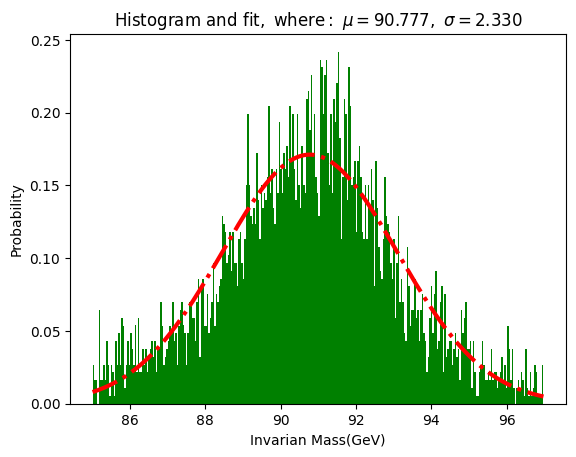
Does the invariant mass follow a normal distribution?

How does cropping the data affect the distribution? (Try to crop the data with different values of min and max)

Why do we need to normalize the data? (Check how the image changes if you remove the normalisation [density])

About transeverse momenta and pseudorapidity

Transeverse momentum \(p_t\) means the momentum which is perpendicular to the beam of particles. It can be calculated from the momenta using vector analysis, but (in most datasets from CMS at least) can be found directly from the loaded data.

Pseudorapidity gives the angle between the particle and the beam, although not using any ‘classical’ angle values. You can see the connection between degree (°) and pseudorapidity in an image a bit later. Pseudorapidity is the column Eta \((\eta)\) in the loaded data.

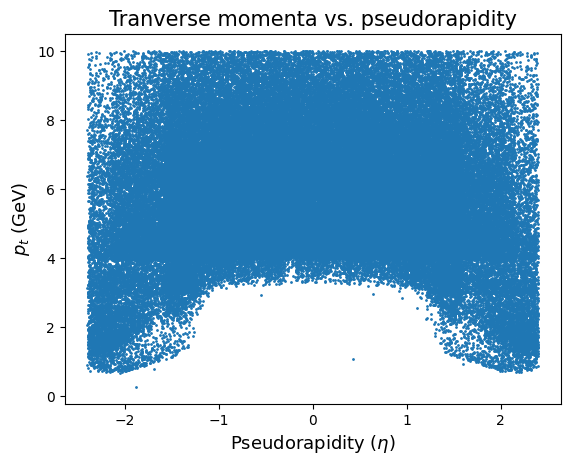
Let us check out what the distribution of transverse momenta looks like.

# allPt now includes all the transverse momenta
allPt = pd.concat([data.pt1, data.pt2]) 

# concat command from the pandas module combines (concatenates) the information into a single column
# (it returns here a DataFrame-type variable, but it only has a singe unnamed column, so later
# we do not have to choose the wanted column from the allPt variable)


# And the histogram
plt.hist(allPt, bins=400, range = (0,50))
plt.xlabel('$p_t$ (GeV)', fontsize = 12)
plt.ylabel('Amount', fontsize = 12)
plt.title('Histogram of transverse momenta', fontsize = 15)

plt.show()

Looks like most of the momenta are between 0 and 10. Let us use this to limit the data we are about to draw.

# we only choose the events below the condition chosen (pt < cond)
cond = 10

smallPt = data[(data.pt1 < cond) & (data.pt2 < cond)]

# Let us save all the etas and pts to variables
allpPt = pd.concat([smallPt.pt1, smallPt.pt2])
allEta = pd.concat([smallPt.eta1, smallPt.eta2])

# and draw a scatterplot

plt.scatter(allEta, allpPt, s=1)

plt.ylabel('$p_t$ (GeV)', fontsize=13)
plt.xlabel('Pseudorapidity ($\eta$)', fontsize=13)
plt.title('Tranverse momenta vs. pseudorapidity', fontsize=15)

plt.show()

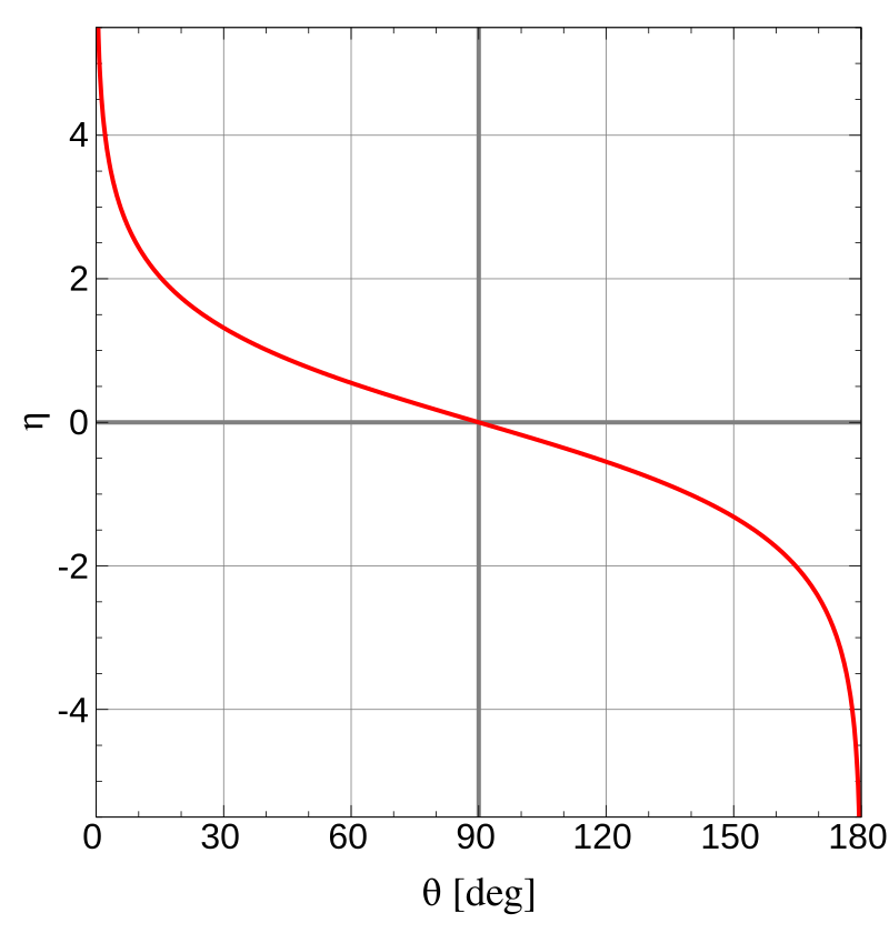
The image on the left shows the relation between pseudorapidity (\(\eta\)) and the angle (\(\theta\)). If \(\eta = 0\), then the event is perpendicular to the beam and so on. Look at this picture and compare it to the plot above and try to answer the questions below.

Some questions

Why is the scatterplot shaped like it is? And why aren’t particles with smaller momentum detected with \(\eta\) being somewhere between -1 and 1?

Why is pseudorapidity an interesting concept in the first place?