The effect of the pseudorapidity on the resolution of the CMS detector TESTI

In this excercise the CMS (Compact Muon Solenoid) detector and the concept of pseudorapidity are introduced. With the real data collected by CMS detector, the effect of the pseudorapidity on the resolution of the CMS detector is observed.

CMS detector

At CERN particles are accelerated and collided with the LHC (Large Hadron Collider) particle accelerator. With the CMS detector, the new particles created in these collisions can be observed and measured. The picture below shows the inside of the CMS detector.

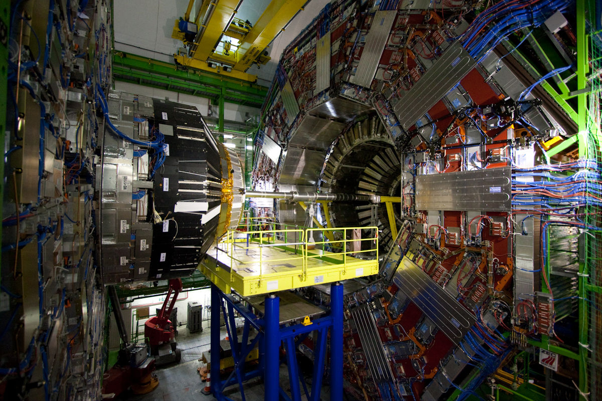(Picture: Domenico Salvagnin, https://commons.wikimedia.org/wiki/File:CMS@CERN.jpg)

Pseudorapidity

In experimental particle physics, pseudorapidity \(\eta\) is a spatial coordinate used to describe the angle between a particle and the particle beam. Pseudorapidity is determined by the equation

\[ \eta \equiv -\ln(\tan(\frac{\theta}{2})), \]

where \(\theta\) is the angle of a particle relative to the particle beam.

In the image below the particle beam would go horizontally from left to right. So with large values of \(\eta\), the direction of a particle created in the collision would differ only a little from the direction of the beam. With small values of \(\eta\) the deflection is larger.

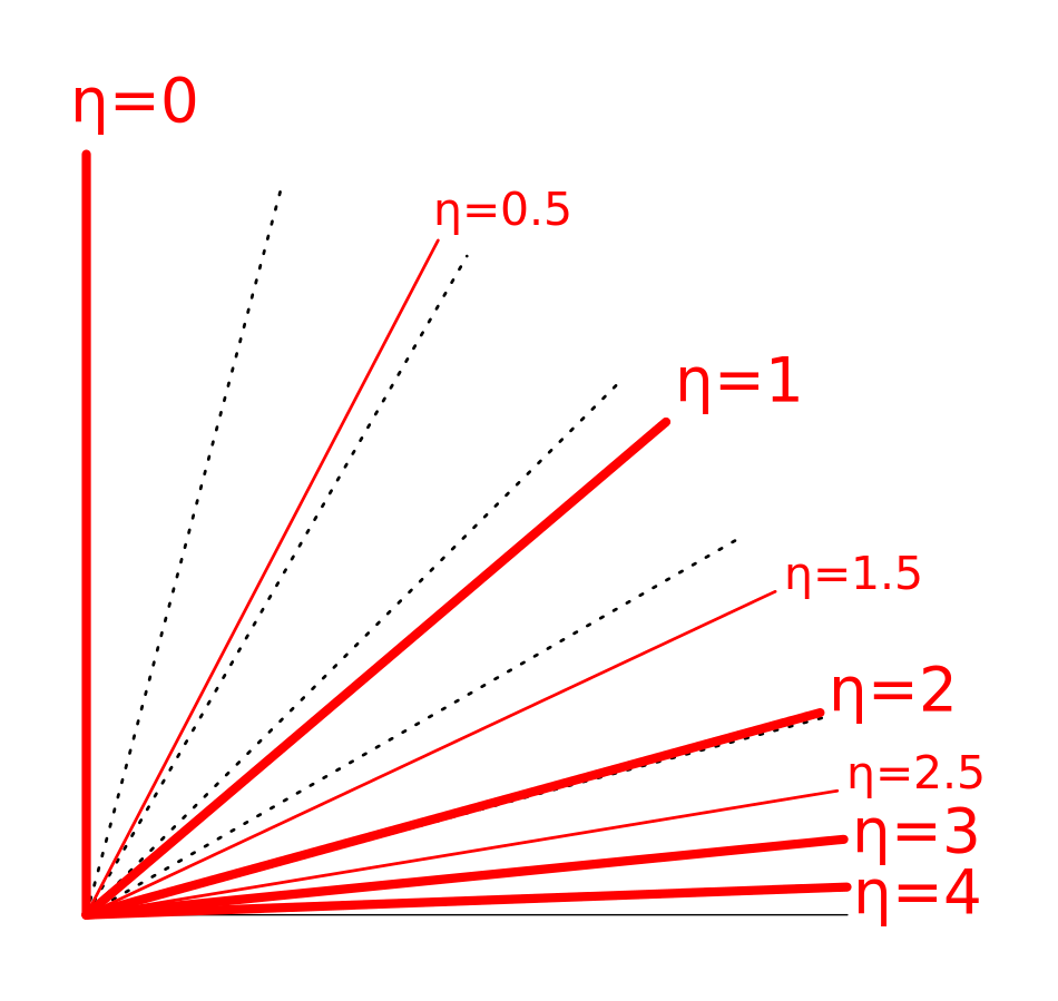
(Image: Wikimedia user Mets501, Own work, CC BY-SA 3.0, https://commons.wikimedia.org/w/index.php?curid=20392149)

The effect of pseudorapidity on the resolution of the measurement

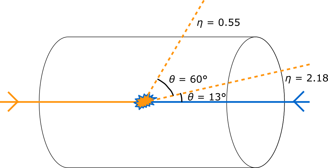
With the CMS detector, the momenta of particles can be measured. Pseudorapidity \(\eta\) affects the resolution of the measurement of momenta, since the particles that hit in the center part of the detector (in the barrel) can be measured more accurately than the particles that hit at the end of the detector (in the endcap).

In the image below there is a draft of the two particles created in the collision event. One hits the barrel of the detector and another hits the endcap. There are also the values of pseudorapidities \(\eta\) and the angles \(\theta\) of the particles.

Let’s start!

Let us start observing how the effect of pseudorapidity on the resolution of the measurement can be seen with the real data collected by the CMS detector.

We will use the data collected in 2011 [1]. From the primary dataset, 10851 collision events where there were exactly two muons have been selected in the file “Zmumu_Run2011A_masses.csv”. (The selection has been done with the code that is openly available at https://github.com/tpmccauley/dimuon-filter.) The measured momenta and energies of the muons are written in the file.

From the measured values of momenta and energies, the invariant mass for muons for every event is calculated. Invariant mass is a mathematical concept, not a physical mass. Invariant mass is determined by the equation

\[ M = \sqrt{(E_1 + E_2)^2-(\vec{p_1} + \vec{p_2})^2}. \]

In the equation, \(E_1\) and \(E_2\) are the energies of the muons and \(\vec{p_1}\) and \(\vec{p_2}\) the momenta of the muons.

If the muon pair comes from the decay of a Z-boson, the invariant mass calculated for that muon pair equals the physical mass of the Z-boson (91.1876 GeV, Particle Data Group). If the two muons originate from some other process (there are a lot of different processes in the particle collisions) then the invariant mass calculated for them is some other value.

Let us observe the invariant masses calculated from different events by plotting a histogram of them. The histogram shows us for how many events the value of the invariant mass is in the desired value range. With the histogram one can see how close to the Z-boson mass (91.1876 GeV) the different invariant mass values will be.


[1] CMS collaboration (2016). DoubleMu primary dataset in AOD format from RunA of 2011 (/DoubleMu/Run2011A-12Oct2013-v1/AOD). CERN Open Data Portal. DOI: 10.7483/OPENDATA.CMS.RZ34.QR6N.

1) Selecting the events

First, we will select from the data the events where the pseudorapidity of the two muons is relatively large (e.g. \(\eta\) > 1.52) and relatively small (e.g. \(\eta\) < 0.45). The selection is made with the code below. We want about the same amount of events in both groups so that a comparison can be made.

# Import the needed modules. Pandas is for the data-analysis, numpy for scientific calculation
# and matplotlib.pyplot for making plots. Modules are named as pd, np and plt.
import pandas as pd
import numpy as np
import matplotlib.pyplot as plt

# Create a new DataFrame structure from the file "Zmumu_Run2011A_masses.csv"
dataset = pd.read_csv('../../Data/Zmumu_Run2011A_masses.csv')

# Set the conditions for large and small etas. These can be changed, but take care that
#the same amount of events is selected for both groups.
cond1 = 1.52
cond2 = 0.45

# Create two DataFrames. Save to the variable "large_etas" events where the pseudorapidities
# of the both muons are larger than "cond1". Save to "small_etas" events where
# the pseudorapidities of the both muons are smaller than "cond2".
large_etas = dataset[(np.absolute(dataset.eta1) > cond1) & (np.absolute(dataset.eta2) > cond1)]
small_etas = dataset[(np.absolute(dataset.eta1) < cond2) & (np.absolute(dataset.eta2) < cond2)]

# Print two empty lines for better design.
print('\n' * 2)

print('The amount of all events = %d' % len(dataset))
print('The amount of events where the pseudorapidity of both muons is large = %d' %len(large_etas))
print('The amount of events where the pseudorapidity of both muons is small = %d' %len(small_etas))

The amount of all events = 10851
The amount of events where the pseudorapidity of both muons is large = 615
The amount of events where the pseudorapidity of both muons is small = 603

2) Creating the histograms

Next we will create separate histograms of the invariant masses for the events with large pseudorapidities and those with small pseudorapidities. With the histograms we can compare these two situations.

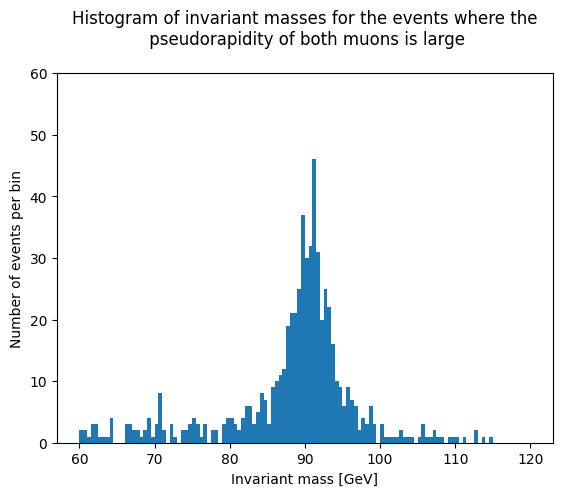
Histogram for the large \(\eta\) events

Let us start with the events where the pseudorapidity of both muons is large.

# Save the invariant masses to variable "inv_mass1".
inv_mass1 = large_etas['M']

# Jupyter Notebook uses "magic functions". With this function it is possible to plot
# the histogram straight to notebook.
%matplotlib inline

# Create the histogram from data in variable "inv_mass1". Set bins and range.
plt.hist(inv_mass1, bins=120, range=(60,120))

# Set y-axis range from 0 to 60.
axes = plt.gca()
axes.set_ylim([0,60])

# Name the axes and give it a title.
plt.xlabel('Invariant mass [GeV]')
plt.ylabel('Number of events per bin')
plt.title('Histogram of invariant masses for the events where the\n pseudorapidity of both muons is large\n')
plt.show()

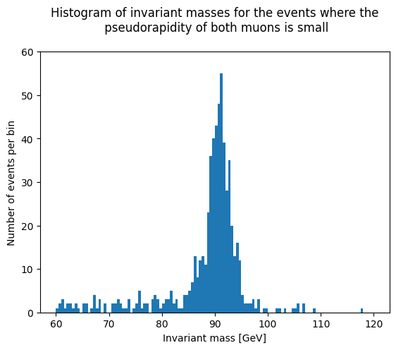
Histogram for the small \(\eta\) events

Analogously, let us plot the histogram of the invariant masses for the events where the pseudorapidity of both muons is small.

# Save the invariant masses to variable "inv_mass2".
inv_mass2 = small_etas['M']

# Jupyter Notebook uses "magic functions". With this function it is possible to plot
# the histogram straight to notebook.
%matplotlib inline

# Create the histogram from data in variable "inv_mass1". Set bins and range.
plt.hist(inv_mass2, bins=120, range=(60,120))

# Set y-axis range from 0 to 60.
axes = plt.gca()
axes.set_ylim([0,60])

# Name the axes and give it a title.
plt.xlabel('Invariant mass [GeV]')
plt.ylabel('Number of events per bin')
plt.title('Histogram of invariant masses for the events where the\n pseudorapidity of both muons is small\n')
plt.show()

3) Exercise

Now we have created from CMS data two histograms of the invariant masses. With the help of the histograms and the theory part of the notebook think about the following questions:

In which way you can see the effect of the pseudorapidity to the measurement resolution of the CMS detector?

Do your results show the same as what the theory predicts?

After answering the questions you can try to change the conditions for the large and small pseudorapidities in the first code cell. The conditions are named cond1 and cond2. Make sure you choose conditions in a way that there will be nearly the same amount of events in both of the groups.

After the changes run the code again. How do the changes affect the number of events? What about the histograms?