What is the Jupyter Notebook?#

1. The basics#

Hey! This platform is the Jupyter Notebook where you can process text, code, images and data interactively. These documents are called “notebooks”.

The Jupyter Notebook works in your internet browser, which means that there is no need to install anything. This makes the notebooks easy to learn and use.

You can also use Jupyter Notebook locally by installing a program on your computer. In that case, a similar window opens up on your on browser, but you can directly use local files or download an unfinished notebook to your computer. This makes sense when you want to make your own exercises or review your students’ answers that include code or data. An example of a program that includes the Jupyter Notebook is Anaconda Navigator.

When using the Jupyter Notebook on a browser, it opens a virtual session that expires if you’re dormant for ten minutes. If restarting doesn’t work, you can save the file after which you can continue making changes.

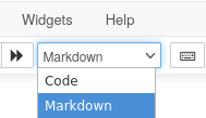
A notebook consists of different cells. We use Markdown cells for text and code cells for executable code. You can modify a cell by double-clicking it. The modified cell can be run by clicking the Run-button or with the shortcut Control + Enter (Mac: Command + Enter). Shift + Enter runs the cell and selects the next one.

You can find everything you need from the toolbar at the top of the window. You can save the file, make checkpoints, add or delete cells, move cells up or down, and run them. You can also choose between a text and a code cell using the drop-down menu.

# This is a code cell. You can write comments or instructions in a code cell by adding a number sign at the beginning of a line.
# Let's do a short calculation for practice:

a = 1+1  # The variable 'a' contains now the calculation 1+1
print(a) # Print the variable 'a' to see result.

Above we have a code cell that contains a short calculation. You can print the result by running the cell. On the left side of the cell there are square brackets. If there reads In [*] inside the brackets, it means that the the execution of the cell is still in progress. When the cell has been run, a number appears inside the square brackets. The numbers tell in which order the cells have been run. If you ran the above cell once, there should be 1 inside the brackets. If you now run the cell for the second time, the number should change to 2.

Variables#

Variables are used to store data, numbers or text for example. A variable has a name and a value.

# name      value 
hedgehog = "suprise!"  # "suprise!" is stored in hedgehog

print(hedgehog)        # without quotes, hedgehog refers to the variable
print("hedgehog")      # with quotes, "hedgehog" is just text

suprise!
hedgehog

Functions#

Functions are used to perform actions without having to write the same code all over again. A funcion has a name, arguments, and (optionally) a return value.

#   name  arguments
def give(food, animal):
    print("You just gave", food, "to", animal)

f1 = "a worm"
f2 = "a fish"
a1 = "a hedgehog"
a2 = "an otter"

# a function is "called" using its name followed by the arguments you want to use
give(f1, a1)
give(f1, a2)

You just gave a worm to a hedgehog
You just gave a worm to an otter

If a function has a return value, it can be stored in a variable.

def triple(number):
    return number * 3  # return value

n = 21
n = triple(n)
print(n)

Exercise: Modify this text cell by adding a sentence that describes today’s weather.#

Exercise: Add a new code cell, calculate a sum, and store it in the variable b.#

2. Python libraries#

When using Python we take use of different libraries, each of which has a unique collection of functions. The libraries we use the most are

numpy, contains tools for numerical analysis
pandas, includes tools for data analysis
matplotlib.pyplot, includes tools for plotting figures

Each library can be imported by using the import command.

Note that sometimes when working with the Binder environment the kernel has to be restarted, which means that you must import the libraries again in order for them to work.

# Run this cell first

import numpy as np  #Import the numpy-library and give it an abbrevation for calling functions
import pandas as pd #Do the same for the other libraries
import matplotlib.pyplot as plt

# Make an array [1 3 6] and save it in the variable 'vector'
vector = np.array([1,3,6])
print(vector)

[1 3 6]

The array function can be used to make vectors and matrices, which makes it great for analyzing data.

# Add 2 to each element.
print(vector + 2)

[3 5 8]

# What is going to happen if we now print only the variable 'vector'?
print(vector)

[1 3 6]

# We need to remember to save our changes to the variable!
vector = vector + 2
print(vector)

[3 5 8]

We can form a matrix by adding arrays as elements in a bigger array.

# Let's form two matrices and try out different sums.
arr1 = np.array([[2,2],
                    [1,2]])
arr2 = np.array([[10,11],
                   [20,21]])
vector_sum = arr1+arr2
print("The sum of the elements of array 1: ", arr1.sum())
print("Vector sums: ", vector_sum)

The sum of the elements of array 1:  7
Vector sums:  [[12 13]
 [21 23]]

3. Reading data#

You can import a dataset into a notebook with an open link. In order to read datasets we need the library pandas (imported as pd above) and the read_csv()-method. The CSV (comma-separated values) file type is useful for saving data into a text file. Using the head()-method we can look at the first five lines of the dataset.

Let’s try this with open data from the CMS experiment at CERN.

data = pd.read_csv("http://opendata.cern.ch/record/5209/files/diphoton.csv")
data.head()

	Run	Event	pt1	eta1	phi1	pt2	eta2	phi2	M
0	199319	641436592	77.2006	0.250438	0.605505	60.1382	0.650821	-1.53900	122.797901
1	199699	336259924	64.1091	0.473667	-0.815133	58.6038	0.032018	2.58568	124.586979
2	201602	114902683	73.7489	0.800788	0.261020	55.9369	0.698872	3.03502	126.462830
3	202087	923352992	102.9550	0.979959	0.148624	76.6940	0.815527	1.67359	123.622542
4	203894	688901524	53.4409	-0.709665	1.642300	46.4314	0.945537	-2.71670	123.203887

You can choose a specific variable from the data in the following way:

# Choosing a specific column
invariant_mass = data['M']
print(invariant_mass)

# Choosing a specific row
row = data.loc[1]
print(row)

0    122.797901
1    124.586979
2    126.462830
3    123.622542
4    123.203887
5    124.444405
6    124.776915
7    125.704971
8    125.691479
9    123.273271
Name: M, dtype: float64
Run      1.996990e+05
Event    3.362599e+08
pt1      6.410910e+01
eta1     4.736670e-01
phi1    -8.151330e-01
pt2      5.860380e+01
eta2     3.201850e-02
phi2     2.585680e+00
M        1.245870e+02
Name: 1, dtype: float64

You can choose another file from the CMS experiment by using the link above and clicking on “CMS” at “Focus on” -part. This opens up a list of datasets for which you can add filters from the left. We recommend you to use the “education” filter in “Filter by keywords”. When you have chosen a file, you can get the direct link to it by right-clicking the download button and selecting “Copy Link”.

Exercise: Open another dataset from the CMS experiment.#

# Write your code here

4. Plotting#

In order to plot functions we need the matplotlib.pyplot library which we imported as plt earlier. We also need the pandas-library for handling data.

Let’s import another dataset and make a histogram of its invariant mass.

dimuon = pd.read_csv("http://cern.ch/opendata/record/545/files/Dimuon_DoubleMu.csv")

#Save the invariant mass in a variable
invariant_mass1 = dimuon['M']

# Plot the histogram with the function hist() of the matplotlib.pyplot module:
# (http://matplotlib.org/api/pyplot_api.html?highlight=matplotlib.pyplot.hist#matplotlib.pyplot.hist).
# 'Bins' determines the number of the bins used.
fig = plt.figure(figsize=(15,10))
plt.hist(invariant_mass1, bins=300)

# Name the axes and give the title
plt.xlabel('Invariant mass [GeV/c²]', fontsize=15)
plt.ylabel('Number of collisions', fontsize=15)
plt.title('The invariant mass of two muons', fontsize=15)

# Show the plot.
plt.show()

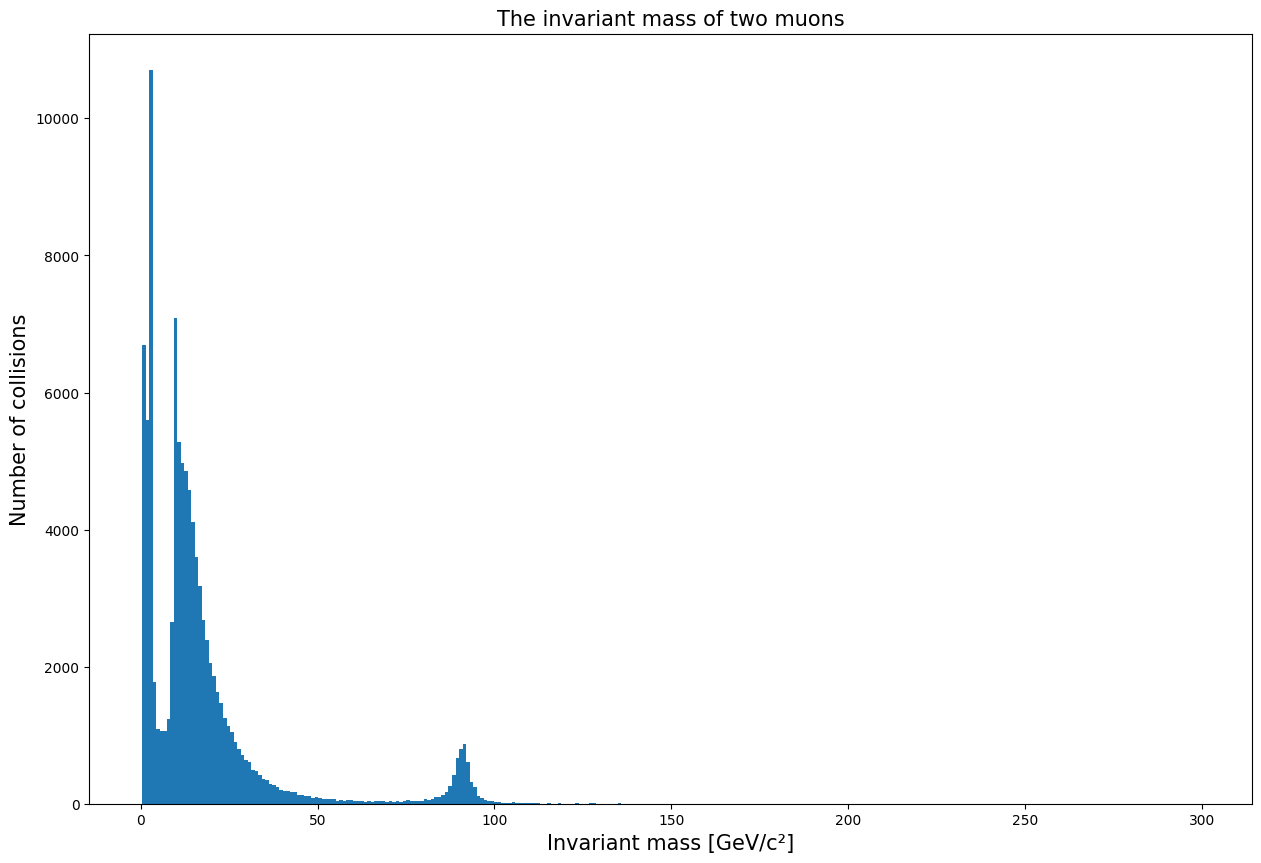
../_images/jupyter-notebook-tutorial_35_0.png

On the plot we can see multiple peaks. We can zoom into them one at a time by adding a “range” argument:

min = 80
max = 100

fig = plt.figure(figsize=(15,10))
plt.hist(invariant_mass1, bins=200, range=[min,max])

# Name the axes and give the title
plt.xlabel('Invariant mass [GeV/c²]', fontsize=15)
plt.ylabel('Number of collisions', fontsize=15)
plt.title('The invariant mass of two muons', fontsize=15)

# Show the plot.
plt.show()

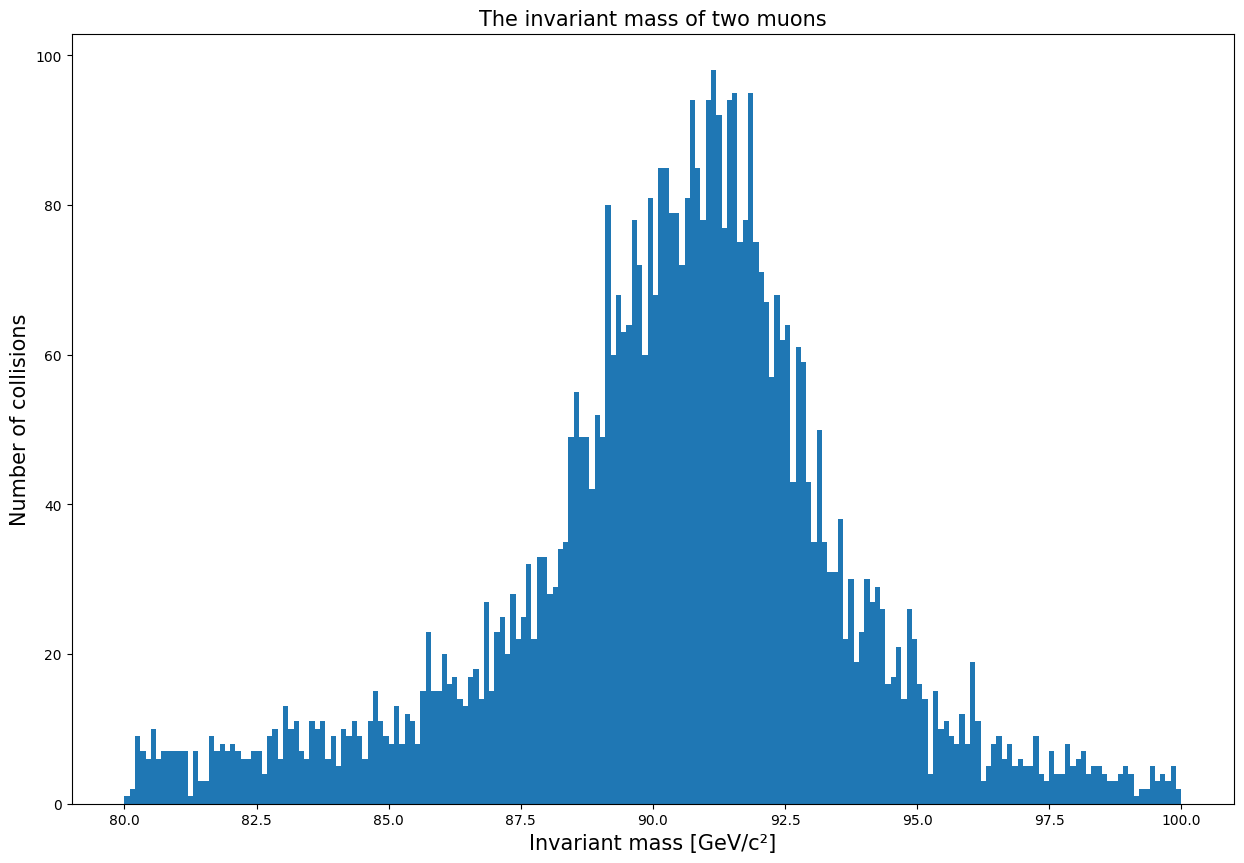
../_images/jupyter-notebook-tutorial_37_0.png

Now we can see more clearly that there is a peak at around 91 GeV. This means that the muons are from a particle that has a mass of 91 GeV. This particle is known as the Z boson.

Exercise: Choose another peak and zoom into it. Do you know which particle it represents?#

5. Additional material#

In the dataset we chose the invariant mass had already been calculated. Often we have to calculate the variable we are interested in ourselves. Let’s now try to calculate the invariant mass of two muons.

The square of the invariant mass of two particles is given by \( M^2 = (E_1+E_2)^2-|| p_1+p_2 ||^2 = (E_1+E_2)^2-((p_{1_x}+p_{2_x})^2+(p_{1_y}+p_{2_y})^2+(p_{1_z}+p_{2_z})^2) \)

Now we can calculate the invariant mass knowing that we can choose the variables by dimuon[‘E1’] etc. Remember that before every complex mathematical function you must define that it comes from the numpy library, which we imported and which we defined as np (e.g. np.sqrt(your_value)).

Additionally, we can use powers without the numpy library using the **-operator (e.g. x^2 is written as x**2).

Exercise: Calculate the invariant mass for all the collisions and save it in the variable ‘invariant_mass2’.#

# Calculate the squared mass here (remove the hash symbol below)
# mass_squared = 

# We must filter out the negative values
invariant_mass2 = np.sqrt(mass_squared[mass_squared>=0])
invariant_mass2.head()

---------------------------------------------------------------------------
NameError                                 Traceback (most recent call last)
Input In [17], in <cell line: 5>()
      1 # Calculate the squared mass here (remove the hash symbol below)
      2 # mass_squared = 
      3 
      4 # We must filter out the negative values
----> 5 invariant_mass2 = np.sqrt(mass_squared[mass_squared>=0])
      6 invariant_mass2.head()

NameError: name 'mass_squared' is not defined

Run the code below to plot a histogram using the values of invariant mass that you calculated. Does it look similar to the one we plotted earlier?

fig = plt.figure(figsize=(15,10))
plt.hist(invariant_mass2, bins=200)

# Name the axes and give the title
plt.xlabel('Invariant mass [GeV/c²]', fontsize=15)
plt.ylabel('Number of collisions', fontsize=15)
plt.title('The invariant mass of two muons', fontsize=15)
#Show the plot.
plt.show()

---------------------------------------------------------------------------
NameError                                 Traceback (most recent call last)
Input In [18], in <cell line: 2>()
      1 fig = plt.figure(figsize=(15,10))
----> 2 plt.hist(invariant_mass2, bins=200)
      4 # Name the axes and give the title
      5 plt.xlabel('Invariant mass [GeV/c²]', fontsize=15)

NameError: name 'invariant_mass2' is not defined

<Figure size 1500x1000 with 0 Axes>

Workshops

What is the Jupyter Notebook?

Contents