Higgs hunting - an example of scientific research

This notebook serves as an example of how many areas of science work by taking a look at how the Higgs boson was discovered.

The data we use here is actual, meaningful data from the CMS experiment that confirmed the existence of this elusive particle, which then resulted in a Nobel prize. Instead of simply presenting it in ready-made graphs, it is now yours to explore. The example is based on the original code in [1] on the CERN Open Data portal, and made into a notebook by Tom McCauley (University of Notre Dame) and Peitsa Veteli (Helsinki Institute of Physics).

The method used is fairly common and useful for many purposes. First, we present some theoretical background, then we make measurements and try to see if those measurements contain something that correlates or clashes with our assumptions. Perhaps the results confirm our expectations, bring up new questions to look into, force us to adapt our theories, or require entirely new ones to explain them. This cycle then continues time and time again.

[1] http://opendata.cern.ch/record/5500 Jomhari, Nur Zulaiha; Geiser, Achim; Bin Anuar, Afiq Aizuddin; (2017). Higgs-to-four-lepton analysis example using 2011-2012 data. CERN Open Data Portal. DOI:10.7483/OPENDATA.CMS.JKB8.RR42

import numpy as np
import pandas as pd
import matplotlib.pyplot as plt

%matplotlib inline

# Data for later use. 

csvs = [pd.read_csv('http://opendata.cern.ch/record/5200/files/4mu_2011.csv'), pd.read_csv('http://opendata.cern.ch/record/5200/files/4e_2011.csv'), pd.read_csv('http://opendata.cern.ch/record/5200/files/2e2mu_2011.csv')]
csvs += [pd.read_csv('http://opendata.cern.ch/record/5200/files/4mu_2012.csv'), pd.read_csv('http://opendata.cern.ch/record/5200/files/4e_2012.csv'), pd.read_csv('http://opendata.cern.ch/record/5200/files/2e2mu_2012.csv')]

fourlep = pd.concat(csvs)

According to the Standard Model, one of the ways the Higgs boson can decay is by first creating two Z bosons that then decay further into four leptons (electrons, muons, etc.). It is not the only process with such a final state, of course, so one has to sift through quite a lot of noise to see that happening. The theory does not say too much about what the mass of Higgs could be, but some clever assumptions and enlightened guesses can get you pretty far. For example, four lepton decay is very dominant in some mass regions, which then guides our search.

# Let us set some values here in regards to the region we are looking at.

rmin = 70
rmax = 181
nbins = 37

M_hist = np.histogram(fourlep['M'], bins = nbins, range = (rmin,rmax))

hist, bins = M_hist
width = 1.0*(bins[1] - bins[0])
center = (bins[:-1] + bins[1:]) / 2

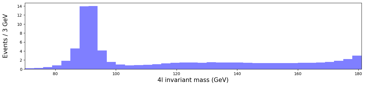
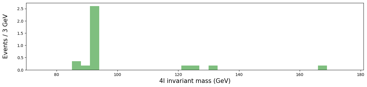
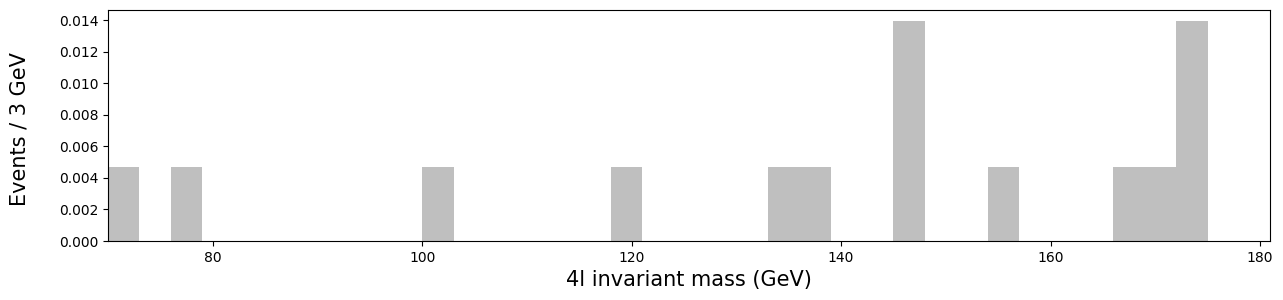
Let us look at some simulations from other processes there. Here are some Monte Carlo -simulated values for such events that have already been weighted by luminosity, cross-section, and number of events. Basically, we create a set of values that have some randomness in them, just like a real measurement would have, but which follows the distribution that has been observed in those processes.

dy = np.array([0,0,0,0,0,0.354797,0.177398,2.60481,0,0,0,0,0,0,0,0,0,0.177398,0.177398,0,0.177398,0,0,0,0,0,0,0,0,0,0,0,0.177398,0,0,0,0])
ttbar = np.array([0.00465086,0,0.00465086,0,0,0,0,0,0,0,0.00465086,0,0,0,0,0,0.00465086,0,0,0,0,0.00465086,0.00465086,0,0,0.0139526,0,0,0.00465086,0,0,0,0.00465086,0.00465086,0.0139526,0,0])
zz = np.array([0.181215,0.257161,0.44846,0.830071,1.80272,4.57354,13.9677,14.0178,4.10974,1.58934,0.989974,0.839775,0.887188,0.967021,1.07882,1.27942,1.36681,1.4333,1.45141,1.41572,1.51464,1.45026,1.47328,1.42899,1.38757,1.33561,1.3075,1.29831,1.31402,1.30672,1.36442,1.39256,1.43472,1.58321,1.85313,2.19304,2.95083])
hzz = np.array([0.00340992,0.00450225,0.00808944,0.0080008,0.00801578,0.0108945,0.00794274,0.00950757,0.0130648,0.0163568,0.0233832,0.0334813,0.0427229,0.0738129,0.13282,0.256384,0.648352,2.38742,4.87193,0.944299,0.155005,0.0374193,0.0138906,0.00630364,0.00419265,0.00358719,0.00122527,0.000885718,0.000590479,0.000885718,0.000797085,8.86337e-05,0.000501845,8.86337e-05,0.000546162,4.43168e-05,8.86337e-05])

Let us take a look at those numbers and how they contribute to what we will measure in the accelerator.

# ZZ, a pair of heavier bosons.

plt.figure(figsize = (15,3))
plt.bar(center, zz, align = 'center', width = width, color = 'b', linewidth = 0, edgecolor = 'black', alpha = 0.5)

plt.xlabel('4l invariant mass (GeV)', fontsize = 15)
plt.ylabel('Events / 3 GeV\n', fontsize = 15)
plt.xlim(rmin,rmax)
plt.show()

# DY, some irreducible background from singular Z bosons.

plt.figure(figsize = (15,3))
plt.bar(center, dy, align = 'center', width = width, color = 'g', linewidth = 0, edgecolor = 'black', alpha = 0.5)

plt.xlabel('4l invariant mass (GeV)', fontsize = 15)
plt.ylabel('Events / 3 GeV\n', fontsize = 15)
plt.xlim(rmin,rmax)
plt.show()

# ttbar, a pair of top and anti-top quarks.

plt.figure(figsize = (15,3))
plt.bar(center, ttbar, align = 'center', width = width, color = 'gray', linewidth = 0, edgecolor = 'b', alpha = 0.5)

plt.xlabel('4l invariant mass (GeV)', fontsize = 15)
plt.ylabel('Events / 3 GeV \n', fontsize = 15)
plt.xlim(rmin,rmax)
plt.show()

Let us stack them together and see what kind of shape we might expect from the experiment.

plt.figure(figsize = (15,5))

# ttbar 
ttbar_bar = plt.bar(center, ttbar, align = 'center', width = width, color = 'gray', linewidth = 0, edgecolor = 'b',
                    alpha = 0.5, label = r'$t\bar{t}$')

# DY
dy_bar = plt.bar(center, dy, align = 'center', width = width, color = 'g', linewidth = 0, edgecolor = 'black',
                 alpha = 0.5, bottom = ttbar, label = 'Z/$\gamma^{*}$ + X')

# ZZ
zz_bar = plt.bar(center, zz, align = 'center', width = width, color = 'b', linewidth = 0, edgecolor = 'black',
                 alpha = 0.5, bottom = ttbar+dy, label = r'ZZ $\rightarrow$ 4l')

plt.title('$ \sqrt{s} = 7$ TeV, L = 2.3 $fb^{-1}$; $\sqrt{s} = 8$ TeV, L = 11.6 $fb^{-1}$ \n', fontsize = 12)
plt.xlabel('$m_{4l}$ (GeV)', fontsize = 15)
plt.ylabel('Events / 3 GeV\n', fontsize = 15)
plt.ylim(0,25)
plt.xlim(rmin,rmax)
plt.legend(fontsize = 15)

plt.show()

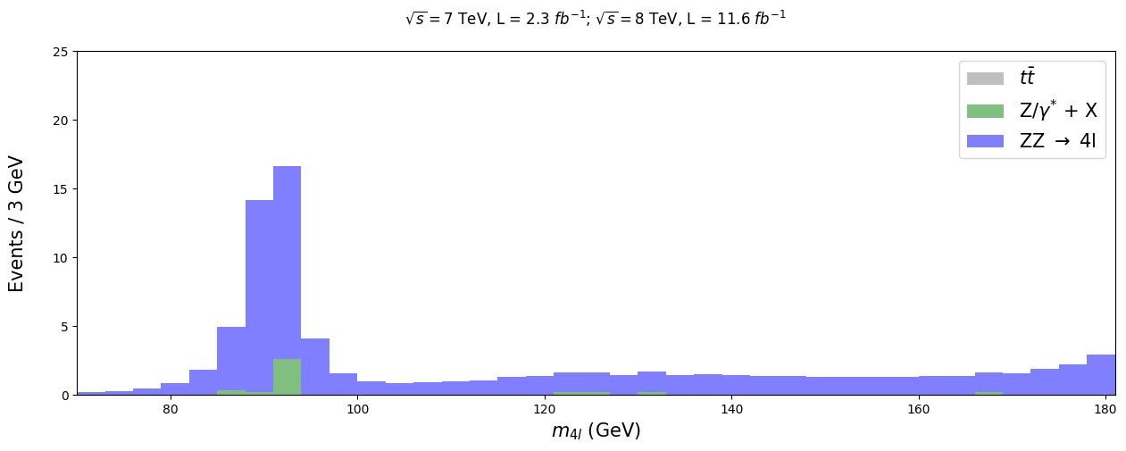
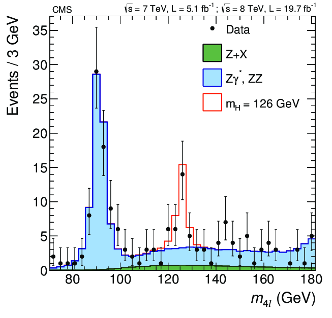
So there ought to be something around 90 GeV or so, which makes sense as most of this comes from Z bosons. Let us add our measured data on top of that. How well do they line up?

plt.figure(figsize = (15,5))

xerrs = [width*0.5 for i in range(0, nbins)]
yerrs = np.sqrt(hist)

# ttbar 
ttbar_bar = plt.bar(center, ttbar, align = 'center', width = width, color = 'gray', linewidth = 0, edgecolor = 'b',
                    alpha = 0.5, label = r'$t\bar{t}$')

# DY
dy_bar = plt.bar(center, dy, align = 'center', width = width, color = 'g', linewidth = 0, edgecolor = 'black',
                 alpha = 0.5, bottom = ttbar, label = 'Z/$\gamma^{*}$ + X')

# ZZ
zz_bar = plt.bar(center, zz, align = 'center', width = width, color = 'b', linewidth = 0, edgecolor = 'black',
                 alpha = 0.5, bottom = ttbar+dy, label = r'ZZ $\rightarrow$ 4l')

# Measured data
data_bar = plt.errorbar(center, hist, xerr = xerrs, yerr = yerrs, linestyle = 'None', color = 'black',
                        marker = 'o', label = 'Data')

plt.title('$ \sqrt{s} = 7$ TeV, L = 2.3 $fb^{-1}$; $\sqrt{s} = 8$ TeV, L = 11.6 $fb^{-1}$ \n', fontsize = 12)
plt.xlabel('$m_{4l}$ (GeV)', fontsize = 15)
plt.ylabel('Events / 3 GeV\n', fontsize = 15)
plt.ylim(0,25)
plt.xlim(rmin,rmax)
plt.legend(fontsize = 15)

plt.show()

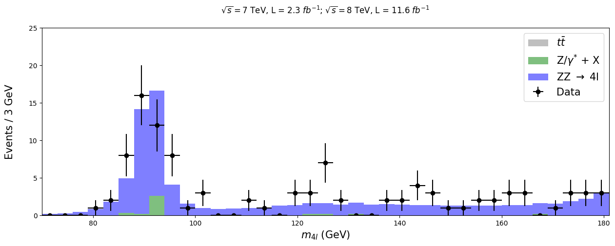
There are clearly some points in there that do not seem to arise in our simulated processes. For comparison’s sake, physicists made distribution simulations for Higgs at varying masses, one of which is shown here. This graph shows us what the Higgs boson should look like, if it had a mass of 125 GeV.

# HZZ, our theoretical assumption of a Higgs via two Z bosons.

plt.figure(figsize = (15,3))
plt.bar(center, hzz, align = 'center', width = width, color = 'w', linewidth = 1, edgecolor = 'r')

plt.xlabel('4l invariant mass (GeV)', fontsize = 15)
plt.ylabel('Events / 3 GeV\n', fontsize = 15)
plt.xlim(rmin,rmax)
plt.show()

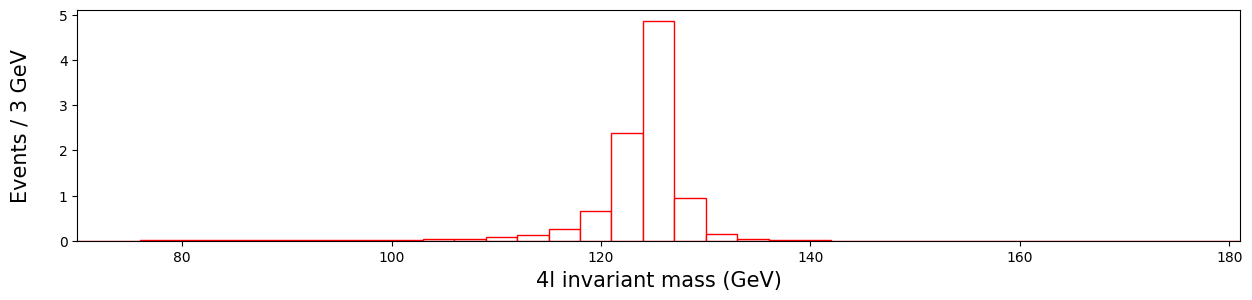
Bonus question: how can something, that seems to have a mass of roughly 125 GeV decay via two Z bosons, with mass over 90 GeV?

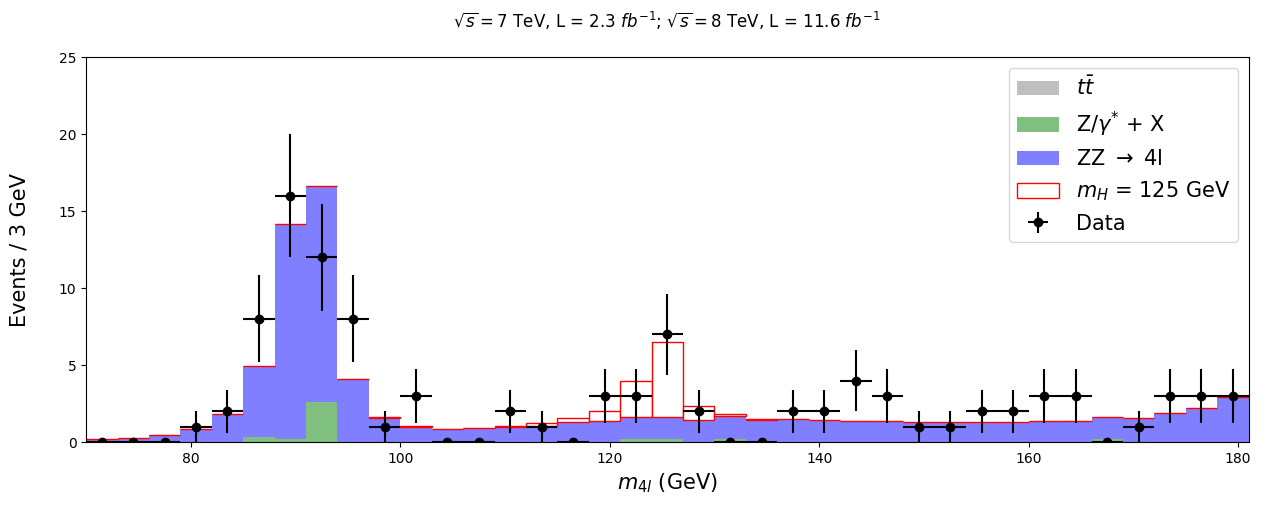
Add that in the previous graph and see how it lines up.

plt.figure(figsize = (15,5))

# ttbar 
ttbar_bar = plt.bar(center, ttbar, align = 'center', width = width, color = 'gray', linewidth = 0, edgecolor = 'b',
                    alpha = 0.5, label = r'$t\bar{t}$')

# DY
dy_bar = plt.bar(center, dy, align = 'center', width = width, color = 'g', linewidth = 0, edgecolor = 'black',
                 alpha = 0.5, bottom = ttbar, label = 'Z/$\gamma^{*}$ + X')

# ZZ
zz_bar = plt.bar(center, zz, align = 'center', width = width, color = 'b', linewidth = 0, edgecolor = 'black',
                 alpha = 0.5, bottom = ttbar+dy, label = r'ZZ $\rightarrow$ 4l')

# HZZ
hzz_bar = plt.bar(center, hzz, align = 'center', width = width, color = 'w', linewidth = 1, edgecolor = 'r',
                  bottom = ttbar+dy+zz, label = '$m_{H}$ = 125 GeV')

# Measured data
data_bar = plt.errorbar(center, hist, xerr = xerrs, yerr = yerrs, linestyle = 'None', color = 'black',
                        marker = 'o', label = 'Data')

plt.title('$ \sqrt{s} = 7$ TeV, L = 2.3 $fb^{-1}$; $\sqrt{s} = 8$ TeV, L = 11.6 $fb^{-1}$ \n', fontsize = 12)
plt.xlabel('$m_{4l}$ (GeV)', fontsize = 15)
plt.ylabel('Events / 3 GeV\n', fontsize = 15)
plt.ylim(0,25)
plt.xlim(rmin,rmax)
plt.legend(fontsize = 15)

plt.show()

This sample seems quite small, and by numerical length it is, but it still gives us an enlightening look at how research is done. There are not very many processes that produce four leptons at the end, so this comprises about half the data that is publicly available from the 2011-2012 run. More precise information about the data can be found here.

# If we take a look at the data, we can see the properties of all four leptons involved.

pd.options.display.max_columns = 50
fourlep.head()

	Run	Event	PID1	E1	px1	py1	pz1	pt1	eta1	phi1	Q1	PID2	E2	px2	py2	pz2	pt2	eta2	phi2	Q2	PID3	E3	px3	py3	pz3	pt3	eta3	phi3	Q3	PID4	E4	px4	py4	pz4	pt4	eta4	phi4	Q4	mZ1	mZ2	M
0	173657	34442568	13	35.9978	32.7631	-4.41922	-14.2436	33.0598	-0.418519	-0.134075	-1	-13	29.0804	-19.31050	-5.31425	21.0837	20.0284	0.918146	-2.873040	1	13	17.3154	-10.87010	-3.64596	12.9753	11.46530	0.971505	-2.81797	-1	-13	11.49390	-1.20978	11.35650	1.29029	11.42070	0.112739	1.676920	1	62.5513	20.5205	91.4517
1	166512	337493970	13	52.9826	-49.9170	8.17082	15.7696	50.5813	0.306925	2.979340	-1	13	72.1018	15.32840	21.35470	-67.1392	26.2866	-1.667150	0.948222	-1	-13	89.7552	10.34670	-20.27240	86.8214	22.76010	2.048740	-1.09888	1	-13	30.21620	2.32913	-13.06840	27.14400	13.27430	1.463510	-1.394420	1	92.1352	90.2049	235.8800
2	171091	69105221	13	165.9750	-12.6280	-30.22890	162.7100	32.7605	2.305880	-1.966510	-1	-13	68.1611	6.93837	22.85760	63.8382	23.8875	1.709440	1.276090	1	-13	19.5056	4.71517	8.50412	16.9087	9.72383	1.320370	1.06454	1	13	24.83870	-8.09683	3.05681	23.28190	8.65464	1.715610	2.780600	-1	58.3874	14.3541	79.3858
3	172952	559839432	13	110.2600	-69.1510	68.83630	-51.3524	97.5720	-0.504613	2.358470	-1	13	88.3199	85.94400	-16.81970	-11.4510	87.5743	-0.130388	-0.193263	-1	-13	45.0987	-19.98280	-29.14080	-28.0247	35.33410	-0.727298	-2.17188	1	-13	9.79377	3.02072	8.34856	-4.13324	8.87824	-0.450186	1.223630	1	91.1877	37.3758	232.9290
4	167282	44166176	-13	54.3881	-27.4999	-43.86520	-16.6628	51.7726	-0.316533	-2.130770	1	13	39.8417	31.53530	18.85330	15.4088	36.7413	0.407975	0.538835	-1	-13	20.3208	3.30081	16.01250	12.0677	16.34910	0.683619	1.36750	1	13	6.83735	4.64276	-2.38618	4.41465	5.22007	0.767963	-0.474752	-1	90.7513	14.7350	119.2900

As we can see, there is certainly some activity going on in the 125 GeV region. This data set is too small to say anything for certain, but it is not too far off from actual analysis results. The most telling differences mainly arise from our somewhat rough methods compared to the more sophisticated ones used at CMS.