Using Python on Jupyter#

This notebook has information about Python and different functions that could be useful for getting started. We have also included some examples about how the functions could be used.

How to use this document: run the cell that imports the needed libraries at the part 2 and then move to the part you’re looking for. Because of this, different functions are defined multiple times in this document in order to mitigate the need to scroll up and down in the notebook.

If you don’t remember how some features work in these notebooks, press the h-button when you haven’t chosen any cells, and you’ll see a list of the shortcuts of Jupyter.

The starting point
Libraries
Data structures and analysis
Basic operations
Generating random values
Plotting figures
Animations
Maps and heat maps
Common problems

1. The starting point#

In programming, you can save different values to variables, which can then be used or changed later. Different variable types are for example the integer (int), floating point number (float), and a string of characters (string). In Python defining new variables is easy since the type of the variable doesn’t have to be defined.

Sometimes the core that runs the code, kernel, has a malfunction. This happens from time to time. When it happens, you can click ‘Kernel’ and ‘Restart & Clear Output’, when the processes and outputs are wiped from the memory. However, doing this doesn’t change the code or text, so it doesn’t fix bugs.

2. Libraries#

Python is a programming language suitable for scientific computing. One of its core principles is the use of different function libraries. These libraries are imported using the import-command.

When you take a look at the materials provided in the Open Data project, you’ll notice that every GitHub folder has a text file “requirements.txt” that enables for example MyBinder to build a workspace for Jupyter. From the file you can see that the most important libraries we’re going to use are:

#The most essential libraries:

import pandas as pd   #contains tools for data analysis
import numpy as np   #contains tools for numerical analysis
import matplotlib.pyplot as plt  #contains tools for plotting figures

#Other useful libraries:

import random as rand   #contains functions for generating pseudo-random numbers
from scipy import stats    #contains scientific computing and statistics sisältää tieteellistä laskentaa ja tilastolaskentaa
from scipy.stats import norm    #tools for analyzing normal distribution
import matplotlib.mlab as mlab  #advanced tools for plotting figures

Remember to run the cell above if you want the examples in this notebook to work. The above could also be written without as-command, which renames the packages, but it enables us to use short names for the libraries, which becomes handy when we use them a lot. If you want to read more about libraries, click on ‘Help’ at the top of the page and you’ll find links for more precise documentation and formatting instructions.

There are many more libraries in Python and you can search for them when you need them. There are thousands of useful examples and materials on the internet, thanks to Python’s large user base. StackExchange and StackOverFlow are great places for searching for answers to your questions.

3. Data structures and analysis#

In short:

Reading a csv-file $\rightarrow$

name = pd.read_csv('path', formatting arguments)

Reading a table $\rightarrow$

pd.read_table('path', formatting arguments)

Getting the first n rows of a table $\rightarrow$

name.head(n)  

Length $\rightarrow$

len(name)  

Shape $\rightarrow$

name.shape 

Column $\rightarrow$

name.column 
name['column'] 

Specifying an interval $\rightarrow$

name[(name.column >= lower_limit) & (name.column <= upper_limit)]  

Searching for text $\rightarrow$

name['column'].str.contains('string')  

Add a column $\rightarrow$

name = name.assign(column = data) 

Remove columns $\rightarrow$

name.drop(['column1','column2'...], axis = 1)

In our exercises the data is often in .csv-form (comma separated values). Data in this form is very easy to read as a table with the use of pandas library. Pandas transforms the csv-file into a two-dimensional DataFrame. You can find more information about it here, where you can also find more information about the different ways you can analyze and process the data.

The easiest ways to read the data are using the functions pd.read_csv and pd.read_table. If data is nice (separated by comma, headers included, etc.), other operations are usually not needed.

#Read a dataset of particle data into a variable and give it a name:

doublemuons = pd.read_csv('http://opendata.cern.ch/record/545/files/Dimuon_DoubleMu.csv')

As you can see, you can read a table straight from a URL-address to a variable. If you have a file in a folder, you can read it using a file path: ‘../folder/file.csv’.

If the data is in some other text form, you can try the more common read_table -command, that understands other tabular texts as well. The most common problem is that the text is separated with something else than comma, such as a tabulator or a semicolon. In that case you can add the argument sep = ‘x’, where x is the character used as a separator. Another common problem is that the headers of the columns aren’t in the first row. In this case we can use the argument header = n, where n is the number of the header row. Note: the numbers start at zero unless otherwise spesified.

More information about the possible arguments here.

Below we have an example of a dataset that doesn’t have a header row. The set contains observations of the Sun from the year 1992 forward. More information about the meaning of each column can be found here.

#Read the dataset and name it:

sun = pd.read_table('http://sidc.oma.be/silso/INFO/sndhemcsv.php', sep = ';', encoding = "ISO-8859-1")

For clarity, let’s see how our data looks like. For this the name.head(n)-command works well. It shows the n first rows of the data. By default n = 5, if you have empty parentheses.

pd.set_option('display.max_columns',None)
doublemuons.head()

	Run	Event	type1	E1	px1	py1	pz1	pt1	eta1	phi1	Q1	type2	E2	px2	py2	pz2	pt2	eta2	phi2	Q2	M
0	165617	74601703	G	9.6987	-9.5104	0.3662	1.8633	9.5175	0.1945	3.1031	-1	G	9.7633	7.3277	-1.1524	6.3473	7.4178	0.7756	-0.1560	1	17.4922
1	165617	75100943	G	6.2039	-4.2666	0.4565	-4.4793	4.2910	-0.9121	3.0350	-1	G	9.6690	7.2740	-2.8211	-5.7104	7.8019	-0.6786	-0.3700	1	11.5534
2	165617	75587682	G	19.2892	-4.2121	-0.6516	18.8121	4.2622	2.1905	-2.9881	-1	G	9.8244	4.3439	-0.4735	8.7985	4.3697	1.4497	-0.1086	1	9.1636
3	165617	75660978	G	7.0427	-6.3268	-0.2685	3.0802	6.3325	0.4690	-3.0992	-1	G	5.5857	4.4748	0.8489	-3.2319	4.5546	-0.6605	0.1875	1	12.4774
4	165617	75947690	G	7.2751	0.1030	-5.5331	-4.7212	5.5340	-0.7736	-1.5522	-1	G	7.3181	-0.3988	6.9408	2.2825	6.9523	0.3227	1.6282	1	14.3159

sun.head()

	1992	01	01.1	1992.001	186	0	186	14.3	1.0	14.3	19	-1	-1.1	1
0	1992	1	2	1992.004	190	18	172	8.2	2.6	7.8	21	-1	-1	1
1	1992	1	3	1992.007	234	26	208	18.3	6.1	17.2	21	-1	-1	1
2	1992	1	4	1992.010	243	54	189	14.8	7.0	13.0	20	-1	-1	1
3	1992	1	5	1992.012	242	58	184	13.8	6.8	12.0	18	-1	-1	1
4	1992	1	6	1992.015	245	79	166	18.7	10.6	15.4	14	-1	-1	1

From the above we can see that the first real row of the sun-variable is used as a header. This is unfortunate because 1) now the headers are misleading and 2) We won’t be able to use the data from the first row in our analysis. Let’s solve the problem by using header = -1, a row that doesn’t exist, as the header argument.

Ylläolevista nähdään, että aurinko-muuttujan ensimmäinen oikea rivi on kaapattu otsikoiksi, mikä on sikäli ikävää että 1) nyt otsikot ovat hämääviä ja 2) meiltä jää yhden rivin verran dataa käsittelemättä jos haluamme vaikkapa kuvaajan taulukon jostain sarakkeesta. Ratkaistaan asia laittamalla dataa ladattaessa otsikointiargumentiksi header = -1, eli rivi jota ei ole olemassa, jolloin kone tuottaa siihen järjestyslukurivin.

sun = pd.read_table('http://sidc.oma.be/silso/INFO/sndhemcsv.php', sep = ';', encoding = "ISO-8859-1", header = None)
sun.head()

	0	1	2	3	4	5	6	7	8	9	10	11	12	13
0	1992	1	1	1992.001	186	0	186	14.3	1.0	14.3	19	-1	-1	1
1	1992	1	2	1992.004	190	18	172	8.2	2.6	7.8	21	-1	-1	1
2	1992	1	3	1992.007	234	26	208	18.3	6.1	17.2	21	-1	-1	1
3	1992	1	4	1992.010	243	54	189	14.8	7.0	13.0	20	-1	-1	1
4	1992	1	5	1992.012	242	58	184	13.8	6.8	12.0	18	-1	-1	1

If we want to change the headers, we can of course name the columns using the argument names = [‘name1’,’name2’,’name3’]

sun = pd.read_table('http://sidc.oma.be/silso/INFO/sndhemcsv.php', sep=';', encoding = "ISO-8859-1", header = None, 
names = ['Year','Month','Day','Fraction','$P_{tot}$','$P_{poh}$','$P_{et}$','$\sigma_{tot}$','$\sigma_{poh}$',
         '$\sigma_{et}$','$N_{tot}$','$N_{poh}$','$N_{et}$','Prov'])
sun.head()

	Year	Month	Day	Fraction	$P_{tot}$	$P_{poh}$	$P_{et}$	$\sigma_{tot}$	$\sigma_{poh}$	$\sigma_{et}$	$N_{tot}$	$N_{poh}$	$N_{et}$	Prov
0	1992	1	1	1992.001	186	0	186	14.3	1.0	14.3	19	-1	-1	1
1	1992	1	2	1992.004	190	18	172	8.2	2.6	7.8	21	-1	-1	1
2	1992	1	3	1992.007	234	26	208	18.3	6.1	17.2	21	-1	-1	1
3	1992	1	4	1992.010	243	54	189	14.8	7.0	13.0	20	-1	-1	1
4	1992	1	5	1992.012	242	58	184	13.8	6.8	12.0	18	-1	-1	1

Among the name.heads() command there are some other small commands that are useful when studying the shape of the data. len(name) tells us the amount of rows, while name.shape tells us the amount of rows and columns.

#Usually the output of a code cell shows only the latest given function. We can output multiple values with the print()-command .
#You can try out what happens if you remove the print()-command.

print (len(sun))
print (sun.shape)

11170
(11170, 14)

Now that data has been imported in a sufficient form, we can start editing it for our own purposes. Usually we are interested in a specific variable within the data, so we must be able to choose specific columns from the original data and choose only the rows in which a certain variable’s values is within some bounds.

A column can be chosen by writing name.column or name[‘column’]. Square brackets are necessary in cases where the name of the column starts with a number, which the machine may interpret as a an ordinal number. If you want to make your life easier and you don’t care about the other columns, it is useful to save the column into a variable with *newName = name.column.

# Save the column that contains the invariant masses in our muon data. The column is named as 'M'.

iMasses = doublemuons.M
iMasses.head()

  17.4922
  11.5534
   9.1636
  12.4774
  14.3159
Name: M, dtype: float64

Selecting rows happens similarly by creating a new variable that contains the elements in the original data that meet the given criteria. For example, choosing an interval would be

newName = name[(name.column >= lower_limit) & (name.column <= upper_limit)]

The condition can be any other logical element, such as a certain number or a piece of text in non-numerical data.

# Let's choose the rows in the particle data where the energy of both particles is more than or equal to 30 GeV.
over30 = doublemuons[(doublemuons.E1 >= 30) & (doublemuons.E2 >= 30)]
over30.head()

	Run	Event	type1	E1	px1	py1	pz1	pt1	eta1	phi1	Q1	type2	E2	px2	py2	pz2	pt2	eta2	phi2	Q2	M
21	165617	74969122	G	59.9226	-46.1516	29.4115	-24.4070	54.7266	-0.4324	2.5742	1	G	52.4465	30.1097	-16.3989	-39.6876	34.2859	-0.9885	-0.4987	-1	89.9557
36	165617	75138253	G	97.1011	-23.6144	6.6660	-93.9497	24.5372	-2.0524	2.8665	-1	G	30.5992	-11.6134	-25.9848	11.2347	28.4619	0.3851	-1.9911	1	88.6081
46	165617	75887636	G	152.9720	7.4657	-30.7098	-149.6710	31.6042	-2.2593	-1.3323	-1	G	33.5835	-9.2878	28.7457	-14.6719	30.2089	-0.4684	1.8833	1	88.2438
78	165617	75833588	G	181.8770	44.1427	-14.9498	175.8040	46.6055	2.0379	-0.3265	1	G	170.0210	-34.6301	12.3248	166.0000	36.7579	2.2128	2.7997	-1	83.0943
110	165617	75779415	G	50.2440	37.8072	-12.2044	-30.7590	39.7283	-0.7124	-0.3122	1	G	49.2396	-47.6064	8.2338	-9.5061	48.3132	-0.1955	2.9703	-1	90.3544

print (len(over30))
print (len(doublemuons))

6516
100000

If we want multiple columns without choosing specific rows, we can write

newVariable = oldVariable[['column1', 'column2', ...]]

If we want to search for a piece of text, we can use te name.loc-function in the following way:

newVariable = oldVariable.loc[oldVariable['column'] == 'piece_of_text']

In that case we would have to know what we are exactly looking for. If you want to find some instances that contain a piece of text, we can use the contains-function. The command

newName= oldName[oldName['column'].str.contains('piece_of_text')]

creates a new variable that has the rows that contain the piece of text we are looking for. By default, the function cares about the letter size, but we can change this by writing

newName= oldName[oldName['column'].str.contains('piece_of_text', case = False)]

Please note that str.contains() in itself is a logical operation that returns true or false from a given question. Negation works as well, such as removing all the joint-stock companies from a list of Finnish alcohol manufacturers (these include ‘Oy’ or ‘Oyj’ in their name).

drinks = pd.read_csv('http://avoindata.valvira.fi/alkoholi/alkoholilupa_valmistus.csv', sep = ';', encoding = "ISO-8859-1", na_filter = False)
drinks.head()

	Y-Tunnus	Nimi	Luvan alkupvm	Olut	Viini	Hedelmäviini	Tislatut alkoholijuomat	Väkiviina	Tilaviinin vähittäismyyntilupa
0	0107011-5	Berner Oy	03.02.2014					X
1	0170318-9	Olvi Oyj	17.02.1995	X		X	X
2	0171079-2	Alahovin Viinitila Oy	25.02.1995	X	X	X	X		X
3	0171110-3	Oy Gust. Ranin Lignell & Piispanen	20.01.1995			X	X
4	0193088-3	Kakslauttanen Arctic Resort Oy	25.02.2020	X

specificManufacturer = drinks[drinks['Nimi'].str.contains('Oy') == False]
print (len(drinks))
print (len(specificManufacturer))

204
35

If you want to add or remove columns from the data, you can use the functions name = name.assign(column = data) and name.drop([‘column1’,’column2’…], axis = 1). In the drop-function setting the axis parameter to 1 tells the function to choose the column.

# Removing a column with the drop-function.

drinks = drinks.drop(['Nimi'], axis = 1)
drinks.head()

	Y-Tunnus	Luvan alkupvm	Olut	Viini	Hedelmäviini	Tislatut alkoholijuomat	Väkiviina	Tilaviinin vähittäismyyntilupa
0	0107011-5	03.02.2014					X
1	0170318-9	17.02.1995	X		X	X
2	0171079-2	25.02.1995	X	X	X	X		X
3	0171110-3	20.01.1995			X	X
4	0193088-3	25.02.2020	X

# Adding a column with the assign-method.
# Let's add a column R that contains numbers.
# The column can contain numbers, text, etc. Just make sure that the column has the right size.

numbers = np.linspace(0, 100, len(drinks))
 
drinks = drinks.assign(R = numbers)
drinks.head()

	Y-Tunnus	Luvan alkupvm	Olut	Viini	Hedelmäviini	Tislatut alkoholijuomat	Väkiviina	Tilaviinin vähittäismyyntilupa	R
0	0107011-5	03.02.2014					X		0.000000
1	0170318-9	17.02.1995	X		X	X			0.492611
2	0171079-2	25.02.1995	X	X	X	X		X	0.985222
3	0171110-3	20.01.1995			X	X			1.477833
4	0193088-3	25.02.2020	X						1.970443

4. Basic operations#

In short:

Absolute value $\rightarrow$

abs(x)  

Addition $\rightarrow$

x + y 

Subtraction $\rightarrow$

x - y  

Division $\rightarrow$

x/y

Multiplication $\rightarrow$

x*y

Power $\rightarrow$

x**y  

Maximum value $\rightarrow$

max(x)  

Minimum value $\rightarrow$

min(x)  

Defining a custom function $\rightarrow$

def name(input):
    operations
    

Square root $\rightarrow$

math.sqrt(x)

np.sqrt(x)

There is nothing extraordinary with the basic operations. If you want the program to print multiple things at once, use the print()-function. Text and numbers can also be combined with the help of the repr(numbers)-function. It returns a printable version of its input. Python has a large number of built-in functions, which you can find from this list. Additionally, here is some information about the built-in types of Python.

# You can modify the content of the 'number'-variable to try out different operations.

number = 14*2+5/2
text = 'The result: '
print (text + repr(number))

The result: 30.5

# max() returns the largest item of an iterable.

someNumbers = [3,6,12,67,578,2,5,12,-34]

print('The largest numbers is ' + repr(max(someNumbers)))

The largest numbers is 578

More interestingly, you can build your own functions in Python. You define the name of the function and its effect by writing

def functionName(input):  
    description indented

# Let's make a function that halves the number it receives as an input.

def halve(a):
    print(a/2)
    
halve(6)

3.0

# Let's make a function that asks users for integers and calculates the sum of them.

def sum_of_inputs(x,y):
    sum_of_two = x + y
    sentence = '{} + {} equals {}.'.format(x, y, sum_of_two)
    print(sentence)
    
def freeChoice():
    a = int(input("Input an integer: "))
    b = int(input("Input another integer: "))
    sum_of_inputs(a, b)

freeChoice() 

---------------------------------------------------------------------------
StdinNotImplementedError                  Traceback (most recent call last)
Input In [19], in <cell line: 13>()
     10     b = int(input("Input another integer: "))
     11     sum_of_inputs(a, b)
---> 13 freeChoice()

Input In [19], in freeChoice()
      8 def freeChoice():
----> 9     a = int(input("Input an integer: "))
     10     b = int(input("Input another integer: "))
     11     sum_of_inputs(a, b)

File /opt/hostedtoolcache/Python/3.8.13/x64/lib/python3.8/site-packages/ipykernel/kernelbase.py:1174, in Kernel.raw_input(self, prompt)
   1167 """Forward raw_input to frontends
   1168 
   1169 Raises
   1170 ------
   1171 StdinNotImplementedError if active frontend doesn't support stdin.
   1172 """
   1173 if not self._allow_stdin:
-> 1174     raise StdinNotImplementedError(
   1175         "raw_input was called, but this frontend does not support input requests."
   1176     )
   1177 return self._input_request(
   1178     str(prompt),
   1179     self._parent_ident["shell"],
   1180     self.get_parent("shell"),
   1181     password=False,
   1182 )

StdinNotImplementedError: raw_input was called, but this frontend does not support input requests.

# Let's make a function that returns a given list of radians as degrees of arc. 
# A while-loop goes through the list and performs an operation on each of the elements.

def radsToDegrees(a):
    i=0
    while i < len(a):
        a[i] = a[i]*360/(2*np.pi)
        i+=1
    return a;

radians = [5,2,4,2,1,3]
radsToDegrees(radians)
print(radians)

[286.4788975654116, 114.59155902616465, 229.1831180523293, 114.59155902616465, 57.29577951308232, 171.88733853924697]

# Or the same with a for-loop:

def radsToDegrees2(a):
    for i in range(0,len(a)):
        a[i] = a[i]*360/(2*np.pi)
    return a;
    
rad = [1,2,3,5,6]
radsToDegrees2(rad)
print(rad)

[57.29577951308232, 114.59155902616465, 171.88733853924697, 286.4788975654116, 343.77467707849394]

5. Generating random values#

In short:

A random integer $\rightarrow$

rand.randint(lower_limit,upper_limit)

A random integer between 0 and 1 $\rightarrow$

rand.random()  

A random collection from a list $\rightarrow$

rand.choices(list, weights, k = count)  

A random collection from a population $\rightarrow$

rand.sample(collection, k = count)  

Normal distribution $\rightarrow$

rand.normalvariate(mean, standard_deviation)  

Evenly spaced numbers $\rightarrow$

np.linspace(start, end, num = the number of samples)  

Evenly spaced numbers $\rightarrow$

np.arange(start, end, stepsize)

Sometimes it is useful to create simulations or random measurements for the analysis. While the development of advanced Monte Carlo simulations is beyond the objectives of this manual, we can take a look at some ways we can produce random numbers. However, it is important to remember that ordinary methods for creating randomness with computers are pseudorandom deterministic processes, and they shouln’t be used for high-secrecy and confidential purposes.

# Create a random integer within a wanted interval.

lottery_ticket = rand.randint(1,100)
text = 'The winning ticket of the day is: '
print(text + repr(lottery_ticket))

The winning ticket of the day is: 7

# Create a random floating point number between 0 and 1 multiplied by 5.

number = rand.random()*5
print(number)

2.486902266233033

# Remove some arbitrary elements from a list, but make some choices more likely than others.

nameForChildren = ['James', 'Anthony', 'Mary', 'Paul', 'Sara','Linda']
weightedProbs = [10,30,20,50,5,5]

# Define how many names we want, k = wanted. Choices-function can take the same results multiple times.

names= rand.choices(nameForChildren, weights = weightedProbs, k = 3)
print(names)

['Paul', 'Paul', 'James']

# Now without duplicates.

students = ['James', 'Anthony', 'Mary', 'Paul', 'Sara','Linda']
threeVolunteers = rand.sample(students, k = 3)
print(threeVolunteers)

['James', 'Anthony', 'Paul']

# A random number from a normal distribution (mean, standard deviation).

number = rand.normalvariate(3,0.1)
print(number)

2.9243753598395763

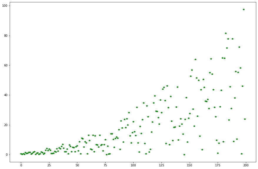
#Let's create an evenly spaced list of numbers between 1 and 10 and randomize it a bit.

listOfNumbers = np.linspace(1, 10, 200)

def randomizer(a):
    b = a.copy()
    
    for i in range(0,len(b)):
        b[i] = b[i]*rand.uniform(0,b[i])
    return b;

result = randomizer(listOfNumbers)
# print(listOfNumbers)
# print(result)

fig = plt.figure(figsize=(15, 10))
plt.plot(result,'g*')
plt.show()

# Another way to produce an evenly spaced array of numbers [a,b[ with the command arange(a,b,c), where c is the stepsize.
# The function may not always work properly if c is not an integer. Note that b is excluded from the array.

# Toinen tapa tuottaa tasaisesti jaettu lukujoukko [a,b[ komennolla arange(a,b,c) missä c on askeleen koko.
# Toiminto voi joskus häröillä jos c ei ole kokonaisluku. Huomaa, että b ei kuulu joukkoon.

numbers = np.arange(1,10,1)
print(numbers)

[1 2 3 4 5 6 7 8 9]

6. Plotting figures#

In short:

Basic plot $\rightarrow$

plt.plot(name, 'style and colour', properties)

Scatterplot $\rightarrow$

plt.scatter(x-data, y-data, marker = 'marker style', color = 'color', properties)

Histogram $\rightarrow$

plt.hist(name, bins, range = (start, end), properties)

Legend $\rightarrow$

plt.legend(properties)

Display all open figures $\rightarrow$

plt.show()

Fit a normal distribution to the data $\rightarrow$

(mu, sigma) = norm.fit(name)

Change the formulation and the name of a figure $\rightarrow$

plt.xlabel('name for the x-label')
plt.title('title')
fig = plt.figure(figsize=(width, height))

Plot the error bars $\rightarrow$

plt.errorbar(value1, value2, xerr = error1, yerr = error2, fmt = 'none')

Figures are perhaps the most important reason to use programming in science education. It is easy and effortless to make clear visualizations of large amounts of data. Different use cases require different methods, the most common of which are presented here.

The colours and markers of figures can freely be changed. Here is a list of markers.

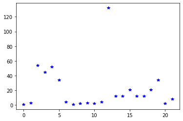
# A basic plot with the plot-function.

numbers = [1,3,54,45,52,34,4,1,2,3,2,4,132,12,12,21,12,12,21,34,2,8]
plt.plot(numbers, 'b*')

# It is a good idea to put plt.show() to the end of plotting. 
# A plot can be seen without it as well, but sometimes it only shows a memory address or some unrecognizable junk. 
# plt.show() fixes this.

plt.show()

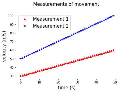
# It is useful to give a figure a name in order to make its purpose clearer.
# Here you can see how different parts of the figure are named.

# Two random datasets:

res1 = np.linspace(10, 20, 50)*rand.randint(2,5)
res2 = np.linspace(10, 20, 50)*rand.randint(2,5)

# Let's plot both of them:

plt.plot(res1, 'r^', label = 'Measurement 1')
plt.plot(res2, 'b*', label = 'Measurement 2')

# Name the axes and the title.

plt.xlabel('time (s)', fontsize = 15)
plt.ylabel('velocity (m/s)', fontsize = 15)
plt.title('Measurements of movement \n', fontsize = 15) # \n creates a new row for formulating the title
          
# Add a legend. If loc-parameter is not specified manually, the legend is automatically placed somewhere where it can fit.

plt.legend(loc='upper left', fontsize = 15)

# Show the plot.

plt.show()

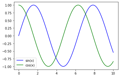
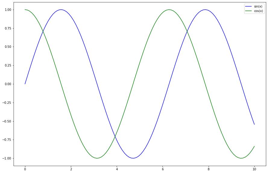
# Other trigonometric functions can be plotted as well.

# The x-axis will be an evenly spaced list of numbers.

x = np.linspace(0, 10, 100)

# Define the functions to be plotted:

y1 = np.sin(x)
y2 = np.cos(x)

# Plot the functions.

plt.plot(x, y1, color = 'b', label = 'sin(x)')
plt.plot(x, y2, color = 'g', label = 'cos(x)')

plt.legend()

plt.show()

# The default size of a figure in Jupyter is somewhat small. The figsize-parameter helps us to scale images to wanted sizes.
# Let's remake the previous figure.

x = np.linspace(0, 10, 100)

y1 = np.sin(x)
y2 = np.cos(x)

# Here is defined the size of the figure. You can try out different sizes.

fig = plt.figure(figsize=(15, 10))

plt.plot(x, y1, color = 'b', label = 'sin(x)')
plt.plot(x, y2, color = 'g', label = 'cos(x)')

plt.legend()

plt.show()

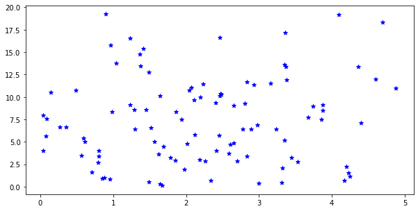
Another common figure is the scatterplot, in which both axes are variables. It is commonly used for example in physics research.

def randomizer(a):
    b = a.copy()
    for i in range(0,len(b)):
        b[i] = b[i]*rand.uniform(0,1)
    return b;

# Take some random data where another variable is spread between 0 to 5 and the other one between 0 to 20.

value1 = randomizer(np.linspace(3,5,100))
value2 = randomizer(np.linspace(10,20,100))

fig = plt.figure(figsize=(10,5))
plt.scatter(value1, value2, marker ='*', color = 'b')
plt.show()

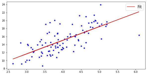
# Another scatterplot example. In this one the values of the variables follow the normal distribution.

def randomize(a):
    b = a.copy()
    for i in range(0,len(b)):
        b[i] = b[i]*rand.normalvariate(1, 0.1)
    return b;

value1 = randomize(np.linspace(3,5,100))
value2 = randomize(np.linspace(10,20,100))

fig = plt.figure(figsize=(10,5))
plt.scatter(value1, value2, marker ='*', color = 'b')

# Let's add a linear fit to the figure using the method of least squares.

slope, intercept, r_value, p_value, std_err = stats.linregress(value1, value2)
plt.plot(value1, intercept + slope*value1, 'r', label='Fit')

plt.legend(fontsize = 15)
plt.show()

# If we wanted to know the mathematical properties of the linear fit, we could for example write print(slope) etc.

# Jos haluaisi tietää suoran matemaattisia arvoja, voisi kirjoittaa esim. print (slope) jne.

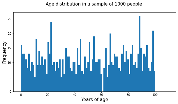
Another important type of diagram is the histogram, which lets us to represent graphically the relative frequencies in the data. Histograms are used everywhere from particle physics to medicine and social science.

# Let's take a random age distribution and make a histogram of it.

def ageGenerator(a):
    b = a.copy()
    for i in range(0, len(b)):
        b[i] = b[i]*rand.randint(1,100)
    return b;

ages = ageGenerator(np.ones(1000))

fig = plt.figure(figsize = (10,5))
plt.hist(ages, bins = 100, range = (0,110))

plt.xlabel('Years of age', fontsize = 15)
plt.ylabel('Frequency', fontsize = 15)
plt.title('Age distribution in a sample of %i people \n' %(len(ages)), fontsize = 15 ) 

plt.show()

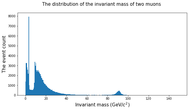
#Let's use some data from a particle physics experiment.

doublemuons = pd.read_csv('http://opendata.cern.ch/record/545/files/Dimuon_DoubleMu.csv')

# Let's make a histogram with respect to the invariant mass, the column M.

fig = plt.figure(figsize = (10,5))
plt.hist(doublemuons.M, bins = 300, range = (0,150))

plt.xlabel('Invariant mass (GeV/$c^2$)', fontsize = 15)
plt.ylabel('The event count', fontsize = 15)
plt.title('The distribution of the invariant mass of two muons \n', fontsize = 15 ) 

plt.show()

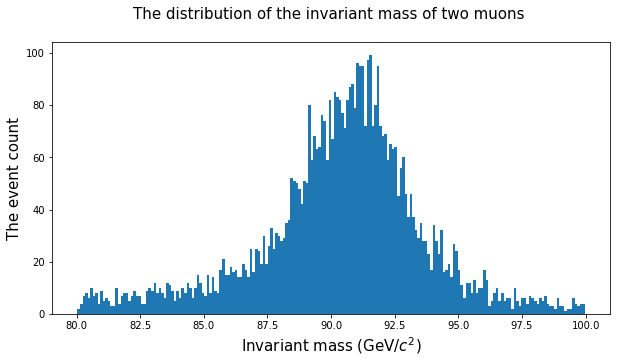
# Let's analyze the area between 80 and 100.

peak = doublemuons[(doublemuons.M >= 80) & (doublemuons.M <= 100)]

fig = plt.figure(figsize = (10,5))
plt.hist(peak.M, bins = 200)

plt.xlabel('Invariant mass (GeV/$c^2$)', fontsize = 15)
plt.ylabel('The event count', fontsize = 15)
plt.title('The distribution of the invariant mass of two muons \n', fontsize = 15 ) 

plt.show()

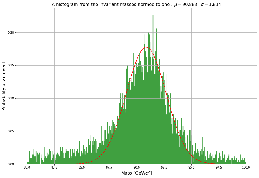
On average, fitting nonlinear curves with the data needs a bit more programming. But in the case of distributions Python offers a variety of suitable functions. For example, you can fit a normal distribution to the above figure as follows:

# Let's defined the limits of the fit:

lower_limit = 87
upper_limit = 95

peak = doublemuons[(doublemuons.M > lower_limit) & (doublemuons.M < upper_limit)]

fig = plt.figure(figsize=(15, 10))

# Let's define the limits for the data we're going to plot.

lower = 80
upper = 100

area = doublemuons[(doublemuons.M > lower) & (doublemuons.M < upper)]

# Since the area of the histogram is set to one for the purposes of the cumulative distribution function,
# let's define a coefficient that takes into account the ratio between the analyzed area and the full area when making a fit.

coef = len(peak)/len(area)
(mu, sigma) = norm.fit(peak.M)

# Let's draw a histogram between the limits we set earlier:

n, bins, patches = plt.hist(doublemuons.M, 300, density = 1, facecolor = 'green', alpha=0.75, histtype='stepfilled',
                            range=(lower,upper))

# Now we'll plot the normal distribution with the coeffiecent we defined above.

y = coef*norm.pdf( bins, mu, sigma)
l = plt.plot(bins, y, 'r--', linewidth=2)

plt.xlabel('Mass [GeV/$c^2$]',fontsize=15)
plt.ylabel('Probability of an event', fontsize=15)

# The title contains the values we calculated from the data.

plt.title(r'$\mathrm{A\ histogram\ from\ the\ invariant\ masses\ normed\ to\ one:}\ \mu=%.3f,\ \sigma=%.3f$'
          %(mu,sigma),fontsize=15)

# Add a grid

plt.grid(True)

plt.show()

We can also plot a figure from a file that doesn’t have numbers. For example, let’s use statistics of road accidents in London.

# Around 40,000 road accidents on different vehicles. The same event has the same reference number AREFNO.

# Nelisenkymmentätuhatta tapaturmaa erinäisin kulkupelein, samalla tapahtumalla on sama viitenumero AREFNO.

traffic = pd.read_table('../exercises/2016-gla-data-extract-vehicle.csv', sep = ",")
injured = pd.read_table('../exercises/2016-gla-data-extract-casualty.csv', sep = ",")

traffic.head()

	AREFNO	Borough	Easting	Northing	Vehicle Ref.	Vehicle Type	Vehicle Type (Banded)	Vehicle Manoeuvres	Vehicle Skidding	Restricted Lane	Junction Location	Veh. Leaving C/W	Veh. Impact	VJNYPURP DECODED	Driver Sex	Driver Age	Driver Age (Banded)
0	1160001090	CITY OF LONDON	531350	181580	1	08 Taxi	4 Taxi	04 Slowing Or Stopping	0 No Skidding/Overturn	0 On Main Cw - Not Rest.	0 Not At Jct	0 Did Not Leave	4 N/S Hit First	1 Jny Part of Work	1 Male	46	35-64
1	1160002980	CITY OF LONDON	532780	180410	1	01 Pedal Cycle	1 Pedal cycle	13 Overtake Move Veh O/S	0 No Skidding/Overturn	0 On Main Cw - Not Rest.	0 Not At Jct	0 Did Not Leave	1 Front Hit First	5 Other/Not Known	3 Not Traced	0	Unknown
2	1160002980	CITY OF LONDON	532780	180410	2	01 Pedal Cycle	1 Pedal cycle	14 Overtake Stat Veh O/S	0 No Skidding/Overturn	0 On Main Cw - Not Rest.	0 Not At Jct	0 Did Not Leave	2 Back Hit First	5 Other/Not Known	1 Male	46	35-64
3	1160006347	CITY OF LONDON	531400	181570	1	09 Car	3 Car	09 Turning Right	0 No Skidding/Overturn	0 On Main Cw - Not Rest.	8 Jct Mid	0 Did Not Leave	1 Front Hit First	5 Other/Not Known	1 Male	22	17-24
4	1160006347	CITY OF LONDON	531400	181570	2	09 Car	3 Car	05 Moving Off	0 No Skidding/Overturn	0 On Main Cw - Not Rest.	8 Jct Mid	0 Did Not Leave	3 O/S Hit First	5 Other/Not Known	1 Male	69	65+

injured.head()

	AREFNO	Borough	Easting	Northing	CREFNO	Casualty Class	Casualty Sex	Casualty Age (Banded)	Casualty Age	No. of Casualties	Casualty Severity	Ped. Location	Ped. Movement	Mode of Travel
0	1160001090	CITY OF LONDON	531350	181580	1	3 Pedestrian	1 Male	25-59	54	1	3 Slight	09 In Road - Not Crossing	7 In Rd Facing Traffic	1 Pedestrian
1	1160002980	CITY OF LONDON	532780	180410	1	1 Driver/Rider	1 Male	25-59	46	1	2 Serious	-2 Unknown	-2 N/A	2 Pedal Cycle
2	1160006347	CITY OF LONDON	531400	181570	3	2 Passenger	2 Female	60+	61	1	3 Slight	-2 Unknown	-2 N/A	4 Car
3	1160006347	CITY OF LONDON	531400	181570	2	1 Driver/Rider	1 Male	60+	69	1	3 Slight	-2 Unknown	-2 N/A	4 Car
4	1160006347	CITY OF LONDON	531400	181570	1	1 Driver/Rider	1 Male	16-24	22	1	3 Slight	-2 Unknown	-2 N/A	4 Car

# Let's choose the age range:

lower_limit = 16
upper_limit = 25
agerange = traffic.loc[(traffic['Driver Age'] <= upper_limit) & (traffic['Driver Age'] >= lower_limit)]

# Let's plot the accidents of this age group on different vehicles.

fig = plt.figure(figsize = (10,5))
plt.hist(agerange['Vehicle Type'], bins = 50)

# Define how the labels in the x-axis work, especially their rotation.

plt.xticks(rotation = 40, ha = 'right')

plt.show()

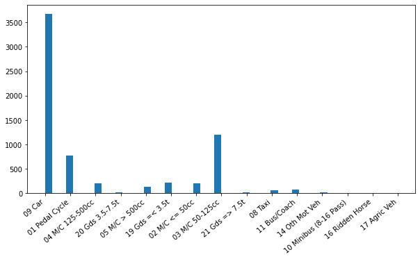
From the figure we can see, unsurprisingly, that most of the road accidents are collisions of cars. However, we can also spot a ridden horse from the list. Let’s analyze this further:

# Isolate the horse collisions from the traffic data.

horses = traffic.loc[traffic['Vehicle Type'] == '16 Ridden Horse']
horses.head()

	AREFNO	Borough	Boro	Easting	Northing	Vehicle Ref.	Vehicle Type	Vehicle Type (Banded)	Vehicle Manoeuvres	Vehicle Skidding	Restricted Lane	Junction Location	Object in C/W	Veh. Leaving C/W	Veh. off C/W	Veh. Impact	VJNYPURP DECODED	Driver Sex	Driver Age	Driver Age (Banded)
33056	0116TW60237	RICHMOND-UPON-THAMES	24	518450	173770	1	16 Ridden Horse	8 Other	18 Going Ahead Other	0 No Skidding/Overturn	0 On Main Cw - Not Rest.	2 Jct Cleared	00 None	0 Did Not Leave	00 None	1 Front Hit First	1 Jny Part of Work	1 Male	25	25-34
33057	0116TW60237	RICHMOND-UPON-THAMES	24	518450	173770	2	16 Ridden Horse	8 Other	18 Going Ahead Other	0 No Skidding/Overturn	0 On Main Cw - Not Rest.	2 Jct Cleared	00 None	0 Did Not Leave	00 None	2 Back Hit First	1 Jny Part of Work	1 Male	28	25-34

# We observe the same AREFNO, which means that the horses collided with each other. What were the injuries?

horseInjuries = injured.loc[injured['AREFNO'] == '0116TW60237']
horseInjuries.head()

	AREFNO	Borough	Boro	Easting	Northing	CREFNO	Casualty Class	Casualty Sex	Casualty Age (Banded)	Casualty Age	No. of Casualties	Casualty Severity	Ped. Location	Ped. Movement	Mode of Travel
22096	0116TW60237	RICHMOND-UPON-THAMES	24	518450	173770	1	1 Driver/Rider	1 Male	25-59	28	1	3 Slight	-2 Unknown	-2 N/A	8 Other Vehicle

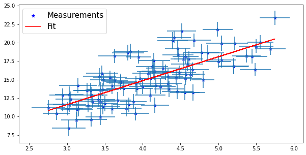
In real data, there are always inaccuracies with respect to the precise measurement and how precisely something can even be measured. These precision values can be obtained using statistical processes or sometimes they are known for each value separately. Let’s take a look at an example of this.

def randomizer(a):
    b = a.copy()
    for i in range(0,len(b)):
        b[i] = b[i]*rand.normalvariate(1, 0.1)
    return b;

# Create data points that vary according to normal distribution.

val1 = randomizer(np.linspace(3,5,100))
val2 = randomizer(np.linspace(10,20,100))

# Give each data point an error that is normally distributed.

err1 = (1/5)*randomizer(np.ones(len(val1)))
err2 = randomizer(np.ones(len(val2)))

fig = plt.figure(figsize=(10,5))
plt.scatter(val1, val2, marker ='*', color = 'b', label = 'Measurements')
plt.errorbar(val1, val2, xerr = err1, yerr = err2, fmt = 'none')

# Let's calculate a linear fit with the sum of least squares.

slope, intercept, r_value, p_value, std_err = stats.linregress(val1, val2)
plt.plot(val1, intercept + slope*val1, 'r', label='Fit')

plt.legend(fontsize = 15)
plt.show()

# If we want to know the mathematical properties of the linear fit, we could for example write print(slope) etc.

7. Animations#

Python has multiple ways of making animations. However, we don’t recommend using the plotly-library with Notebooks, since it is so slow. The following example shows clearly why more data gives better results.

# Import the data we want to use
data = pd.read_csv('http://opendata.cern.ch/record/545/files/Dimuon_DoubleMu.csv')

# Save the invariant mass into a variable
iMass = data.M

# Define a function that produces our figure. 
# Num says how many steps we have taken and the function draws a new histogram for each step.

def updt_hist(num, iMass):
    plt.cla()
    axes = plt.gca()
    axes.set_ylim(0,12000)
    axes.set_xlim(0,200)
    plt.hist(iMass[:num*480], bins = 120)

Note that cells that contain animations are slow. The more images, the slower it is to make them. This can take several minutes.

# Import a library that produces animations.
import matplotlib.animation

%%capture

# The purpose of the %%capture -magic function is to prevent this cell from displaying a finished image, 
# so that there won't be empty images or other unnecessary things. It makes our life easier.

fig = plt.figure()

# fargs says which variables a function takes as input and the empty part tells to the prorgram that it must use two variables.
# The other variable is the current frame.

anim = matplotlib.animation.FuncAnimation(fig, updt_hist, frames = 200, fargs=(iMass, ) )

# anim.to_jshtml() changes the animation to (javascript)html so that Notebook can show it.

from IPython.display import HTML
HTML(anim.to_jshtml())

# Tämän ajamalla animaatio saadaan sitten näkyväksi, kun se on ohjelman muistissa.
# Running this cell the animation can be shown, when it is in the memory of the program.

HTML(anim.to_jshtml())

8. Maps and heat maps#

Let’s now take a look at interactive maps that utilize data! Making them is easier than you would think. In the following example we use data that contains latitudes and longitudes.

# We can find different maps from the folium-library.

import folium

# Tiheyttä värein edustava heatmap-systeemi on myös näppärä, joten otetaan se käyttöön.
# Let's import the HeatMap-system. It is represents density as colours, which is useful for our purposes.

from folium.plugins import HeatMap

# This dataset contains information about earthquakes all around the world that happened in the last month. 
# It is updated continually.

quakeData = pd.read_csv('https://earthquake.usgs.gov/earthquakes/feed/v1.0/summary/all_month.csv')
quakeData.head()

# Since our data is in DataFrame-form, we change it first into lists that HeatMap understands.

dat = [0]*len(quakeData)

# The list contains values (tuples), that contain latitude, longitude and the strength of the earthquake.
# Magnitude isn't strictly necessary for our purposes, but it can become useful for example if we want to study 
# only the instances that cross a certain threshold.

for i in range(0, len(quakeData)):
    dat[i] = [quakeData['latitude'][i], quakeData['longitude'][i], quakeData['mag'][i]]

# In case that there are also rows whose magnitude is unknown (indicated as NaN),
# let's remove them so that our list doesn't start behaving awkwardly.

dat = [x for x in dat if ~np.isnan(x[2])]

# Different types of maps: https://deparkes.co.uk/2016/06/10/folium-map-tiles/
# 'world_copy_jump = True' enables rolling the map to the side so that the earthquakes are still shown.
# If you only want one map projection, please add the argument 'no_wrap = True' to the list of arguments.
# The argument control_scale adds a scale to the map.

m = folium.Map([15., -75.], tiles='openstreetmap', zoom_start=3, world_copy_jump = True, control_scale = True)

HeatMap(dat, radius = 15).add_to(m)

m

9. Common problems#

Here is a list of some common problems:

A cell got stuck and it won’t draw my figure or run my code.
An error message says ‘name is not defined’ or ‘name does not exist’.
I’m trying to save something in a variable but print(name) outputs None.
I can’t load my data into a variable.
Why does my dataset have ‘NaN’-values?
I combined pieces of data into a variable, but I can’t use it.
Why doesn’t my code work although I know it’s written correctly?
The dates in the data mess up the program. How do I fix this?
I copied the data into a new variable. After I have processed it, I see that the values of the original variable have changed.

Solu jäi jumiin eikä piirrä kuvaajaani tai aja koodiani?
Virheilmoitus herjaa ‘nimi is not defined’ tai ‘nimi does not exist’?
Yritän tallentaa muuttujaan asioita, mutta print(nimi) kertookin None?
Datani ei suostu lataamaan?
Lataamassani datassa on jotain omituisia ‘NaN’-arvoja?
Yhdistin palasia datasta, mutta nyt en enää pysty tekemään asioita uudella muuttujallani?
Koodini ei toimi, vaikka se on ihan varmasti oikein kirjoitettu?
Datan päivämäärät sekoittavat toiminnan, miten korjaan?
Kopioin datan uuteen muuttujaan, jonka käsittelyn jälkeen huomaan alkuperäisen muuttujan arvojen vaihtuneen?

A cell got stuck and it won’t draw my figure or run my code.#

If it takes more time than it should to run a cell, and the code isn’t doing anything computing-intensive, then it is possible that there is an infinite loop in the code. Stop the execution of the kernel and make sure your code doesn’t have infinite loops. If you don’t find the problem, make the syntax simpler so that you can be sure that the code is logical.

A common problem is that a syntax error drives the machine to do something wrong. An example: you’re making a histogram of a column of a big data set but you forget to add the name of the column into your code. Now the machine tries to execute your command and gets confused about a table that contains the whole data. Stop the kernel and change the names of the variables.

An error message says ‘name is not defined’ or ‘name does not exist’.#

The variable you’re alluding to doesn’t exist. Are you sure you have run the cell where the variable is defined in this session? Also, remember that the size of the letters matters.

I’m trying to save something in a variable but print(name) outputs None.#

You probably haven’t saved the value properly into the variable. Remember to save all the operations you have made into a variable, e.g.

variable = ... imported data
variable = variable*2

and not

variable = ... imported data
variable*2

If print(variable) returns None, the variable is empty. Make sure that the operation you want to do is possible and doesn’t fall apart because of e.g. invalid inputs for an inner function.

I can’t load my data into a variable.#

Ordinary csv-files and similar files can be viewed with text editors. There you can see which character separates the values, which row the relevant data starts from, and is does the file contain the data you need.

Separator characters, headers, and others can be defined as parameters of the read-function, e.g.

pd.read_csv('link to a file', sep = ';')

reads a csv-file whose values are separated by a semicolon. More about this in the section 3.

pd.read_table() can help to clarify the data if you don’t want to open a text editor.

Sometimes there are incompabilities with the codes that guide the character encoding. This is when the parameter encoding can be of help. More information about them can be found here. If the default option doesn’t work, try some variant of ISO; it should work in most cases.

Why does my dataset have ‘NaN’-values?#

NaN, ‘Not a Number’, says that there is no value in this part of the data set. Either the value is weird (such as the square root of a negative number), or it just doesn’t exist.

Many functions doen’t care about NaN-values or you can add a parameter that lets the function to ignore them. This helps especially when you have big datasets, since the program won’t stall when it has to compute something incalculable.

I combined pieces of data into a variable, but I can’t use it.#

Did you combine different types of variables? The computer handles integers, floating point numbers, strings, and other value types differently. Sometimes a series of numbers is written as a string into a dataset, which causes all kind of trouble. Python has different commands for checking the type of a variable, such as isstring.

Did you combine the pieces correctly? If you wanted columns next to each other, make sure you didn’t combine them into a single long column. Analyzing the data with e.g. commands len(name) and name.head() is often useful in these situations.

Why doesn’t my code work although I know it’s written correctly?#

Go over your code and check that there isn’t a dot in a wrong place or a wrong size letter somewhere.

If you’re sure the code is supposed to work but it doesn’t, the problem may be caused by old values in the kernel’s memory. Try clicking on ‘Restart & Clear Output’ from the Kernel-menu, possibly even couple times.

The dates in the data mess up the program. How do I fix this?#

Dates can be expressed in many forms in the data. If the default settings don’t work, you can find different parameters that affect the interpretation of dates in the documentation of pd.read_csv(). For example. dayfirst or date_parser may solve the problem. Python has also the time-library that can be of help.

I copied the data into a new variable. After I have processed it, I see that the values of the original variable have changed.#

Python operates by pointers. This means that a variable contains a pointer to a memory slot where the information is located, rather than containing the information itself. When copying a full data variable to a new variable rather than single rows or columns, it may happen that the new variable just points to the old information. If the content of the new variable is changed, the changes are made to the old variable as well. Because of this, it is useful to copy the original variable as follows:

newName = oldName.copy()

Now the program uses a new memory slot so that the new variable doesn’t point to the old one. The problem seems to happen only when saving the whole data into a new variable, which means that isolating single rows or columns into variables happens without referencing the original data.

Python and Jupyter

Using Python on Jupyter

Contents

Using Python on Jupyter#

1. The starting point#

2. Libraries#

3. Data structures and analysis#

4. Basic operations#

5. Generating random values#

6. Plotting figures#

7. Animations#

8. Maps and heat maps#

9. Common problems#

A cell got stuck and it won’t draw my figure or run my code.#

An error message says ‘name is not defined’ or ‘name does not exist’.#

I’m trying to save something in a variable but print(name) outputs None.#

I can’t load my data into a variable.#

Why does my dataset have ‘NaN’-values?#

I combined pieces of data into a variable, but I can’t use it.#

Why doesn’t my code work although I know it’s written correctly?#

The dates in the data mess up the program. How do I fix this?#

I copied the data into a new variable. After I have processed it, I see that the values of the original variable have changed.#